You are viewing the documentation for an older COMSOL version. The latest version is available here.
PDF

One-Sided Magnet and Plate
Introduction
Permanent magnets with a one-sided flux are used to attach posters and notes to refrigerators and notice boards but can also be found in advanced physics applications like particle accelerators. The one-sided flux behavior is obtained by giving the magnet a magnetization that varies in the lateral direction (Ref. 1). As no currents are present, it is possible to model a permanent magnet using a scalar magnetic potential formulation. This application shows this technique to model a cylindrical one-sided permanent magnet. A special technique to model thin sheets of high permeability material was used to model a thin μ-metal plate next to the magnet. This circumvents the difficulty of volumetric meshing of thin extended structures in 3D.
Figure 1: A cylindrical magnet above a μ-metal plate is modeled.
Model Definition
In a current free region, where
you can define the scalar magnetic potential, Vm, from the relation
This is analogous to the definition of the electric potential for static electric fields.
Using the constitutive relation between the magnetic flux density and magnetic field
together with the equation
you can derive the following equation for Vm:
It can be shown that applying a laterally periodic magnetization of
results in a magnetic flux that only emerges on one side of the magnet.
Boundaries
Along the exterior boundaries, the magnetic field should be tangential to the boundary as the flow lines should form closed loops around the magnet. The natural boundary condition from the equation is
Thus the magnetic field is made tangential to the boundary by a Neumann condition on the potential. On the interior boundary representing the μ-metal plate, you apply a special boundary condition for thin sheets of highly permeable material. Such plates are often used for the purpose of magnetic shielding.
Magnetic saturation effect in the Plate
Magnetic saturation effects are important in many applications. In a second step, the instructions show how to include a nonlinear magnetic material with saturation in the plate.
Force Calculation
To calculate the force on the plate, use the surface stress tensor
where n1 is the boundary normal pointing out from the plate and T2 the stress tensor for air.
In this model the H and B fields are discontinuous across the plate, which makes it necessary to evaluate the fields on both sides of the plate
Results and Discussion
Figure 2 shows the calculated magnetic flux density and direction for the version of the one-sided magnet that includes magnetic saturation in the plate. Saturation effects cause a drop in the force on the plate. A comparison also shows that the force is considerably higher for the case with the one-sided magnetization compared to the case with a uniform magnetization of the same amplitude.
Figure 2: The magnetic flux density and direction is plotted in a cross section of the geometry.The one-sided behavior is apparent, as the flux does not emerge on the top of the magnet. The differential relative permeability in the plate is shown on a separate scale illustrating that it is driven well into saturation.
Reference
1. H.A. Shute, J.C. Mallinson, D.T. Wilton, and D.J. Mapps, “One-Sided Fluxes in Planar, Cylindrical and Spherical Magnetized Structures,” IEEE Transactions on Magnetics, vol. 36, no. 2, pp. 440–451, 2000.
Application Library path: ACDC_Module/Magnetostatics/one_sided_magnet
Modeling Instructions
From the File menu, choose New.
New
In the New window, click  Model Wizard.
Model Wizard
1
In the Model Wizard window, click  3D.
2
In the Select Physics tree, select AC/DC>Magnetic Fields, No Currents>Magnetic Fields, No Currents (mfnc).
3
Click Add.
4
Click  Study.
5
In the Select Study tree, select General Studies>Stationary.
6
Global Definitions
Parameters 1
1
In the Model Builder window, under Global Definitions click Parameters 1.
2
In the Settings window for Parameters, locate the Parameters section.
3
Geometry 1
1
In the Model Builder window, under Component 1 (comp1) click Geometry 1.
2
In the Settings window for Geometry, locate the Units section.
3
From the Length unit list, choose mm.
Cylinder 1 (cyl1)
1
In the Geometry toolbar, click  Cylinder.
2
In the Settings window for Cylinder, locate the Size and Shape section.
3
In the Radius text field, type 10.
4
In the Height text field, type 5.
5
In the Geometry toolbar, click  Build All.
6
Click the  Zoom Extents button in the Graphics toolbar.
Work Plane 1 (wp1)
1
In the Geometry toolbar, click  Work Plane.
2
In the Settings window for Work Plane, locate the Plane Definition section.
3
In the z-coordinate text field, type -5.
Work Plane 1 (wp1)>Plane Geometry
In the Model Builder window, click Plane Geometry.
Work Plane 1 (wp1)>Circle 1 (c1)
1
In the Work Plane toolbar, click  Circle.
2
In the Settings window for Circle, locate the Size and Shape section.
3
In the Radius text field, type 10.
4
In the Work Plane toolbar, click  Build All.
5
Click the  Zoom Extents button in the Graphics toolbar.
6
In the Model Builder window, right-click Geometry 1 and choose Build All.
7
Click the  Zoom Extents button in the Graphics toolbar.
Sphere 1 (sph1)
1
In the Geometry toolbar, click  Sphere.
2
In the Settings window for Sphere, locate the Size section.
3
In the Radius text field, type 20.
4
Click  Build All Objects.
5
Click the  Wireframe Rendering button in the Graphics toolbar.
6
Click the  Zoom Extents button in the Graphics toolbar.
Next will be some selections. These selections will be used later on, when assigning domain features or building the mesh for instance.
Definitions
Air
1
In the Definitions toolbar, click  Explicit.
2
In the Settings window for Explicit, type Air in the Label text field.
3
Magnet
1
In the Definitions toolbar, click  Explicit.
2
In the Settings window for Explicit, type Magnet in the Label text field.
3
Plate
1
In the Definitions toolbar, click  Explicit.
2
In the Settings window for Explicit, type Plate in the Label text field.
3
Locate the Input Entities section. From the Geometric entity level list, choose Boundary.
4
Materials
Air
1
In the Model Builder window, under Component 1 (comp1) right-click Materials and choose Blank Material.
2
Right-click Material 1 (mat1) and choose Rename.
3
In the Rename Material dialog box, type Air in the New label text field.
4
5
In the Settings window for Material, locate the Geometric Entity Selection section.
6
From the Selection list, choose Air.
7
Locate the Material Contents section. In the table, enter the following settings:
Linear mu-metal
1
In the Model Builder window, right-click Materials and choose Blank Material.
2
Right-click Material 2 (mat2) and choose Rename.
3
In the Rename Material dialog box, type Linear mu-metal in the New label text field.
4
5
In the Settings window for Material, locate the Geometric Entity Selection section.
6
From the Geometric entity level list, choose Boundary.
7
From the Selection list, choose Plate.
8
Click to expand the Material Properties section. In the Material properties tree, select Basic Properties>Relative Permeability.
9
Click  Add to Material.
10
Locate the Material Contents section. In the table, enter the following settings:
Magnetic Fields, No Currents (mfnc)
Magnetic Flux Conservation 2
1
In the Model Builder window, under Component 1 (comp1) right-click Magnetic Fields, No Currents (mfnc) and choose Magnetic Flux Conservation.
2
In the Settings window for Magnetic Flux Conservation, locate the Constitutive Relation B-H section.
3
From the Magnetization model list, choose Magnetization.
4
Locate the Domain Selection section. From the Selection list, choose Magnet.
5
Locate the Constitutive Relation B-H section. Specify the M vector as
The specified magnetization will result in a magnetic flux that only emerges from the lower side of the magnet.
Magnetic Shielding 1
1
In the Physics toolbar, click  Boundaries and choose Magnetic Shielding.
2
In the Settings window for Magnetic Shielding, locate the Boundary Selection section.
3
From the Selection list, choose Plate.
4
Locate the Magnetic Shielding section. In the ds text field, type 0.5[mm].
So far the magnetic potential is not constrained anywhere and the solution can only be computed up to a constant. Add a condition to fix a specific value on a point.
Zero Magnetic Scalar Potential 1
1
In the Physics toolbar, click  Points and choose Zero Magnetic Scalar Potential.
2
Mesh 1
1
In the Model Builder window, under Component 1 (comp1) right-click Mesh 1 and choose Build All.
2
Click the  Zoom Extents button in the Graphics toolbar.
The default mesh is sufficient for the time being. We will refine it later.
Study 1
1
In the Model Builder window, click Study 1.
2
In the Settings window for Study, locate the Study Settings section.
3
Clear the Generate default plots check box.
4
In the Home toolbar, click  Compute.
Results
3D Plot Group 1
In the Home toolbar, click  Add Plot Group and choose 3D Plot Group.
Slice 1
1
Right-click 3D Plot Group 1 and choose Slice.
2
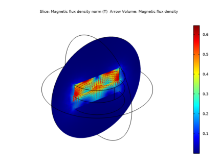
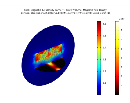
In the Settings window for Slice, click Replace Expression in the upper-right corner of the Expression section. From the menu, choose Component 1 (comp1)>Magnetic Fields, No Currents>Magnetic>mfnc.normB - Magnetic flux density norm - T.
3
Locate the Plane Data section. From the Plane list, choose zx-planes.
4
In the Planes text field, type 1.
5
In the 3D Plot Group 1 toolbar, click  Plot.
6
Click the  Zoom Extents button in the Graphics toolbar.
Arrow Volume 1
1
In the Model Builder window, right-click 3D Plot Group 1 and choose Arrow Volume.
2
In the Settings window for Arrow Volume, locate the Arrow Positioning section.
3
Find the x grid points subsection. In the Points text field, type 50.
4
Find the y grid points subsection. In the Points text field, type 1.
5
Find the z grid points subsection. In the Points text field, type 50.
6
In the 3D Plot Group 1 toolbar, click  Plot.
7
Click the  Zoom In button in the Graphics toolbar.
The arrow plot shows the magnetic flux density and the surface plot shows its norm.
Having plotted the magnetic flux density, proceed to visualize the magnetic field on the plate.
Study 1/Solution 1 (sol1)
In the Model Builder window, expand the Results>Datasets node, then click Study 1/Solution 1 (sol1).
Selection
1
In the Results toolbar, click  Attributes and choose Selection.
2
In the Settings window for Selection, locate the Geometric Entity Selection section.
3
From the Geometric entity level list, choose Boundary.
4
From the Selection list, choose Plate.
Surface 1
1
In the Model Builder window, right-click 3D Plot Group 1 and choose Surface.
2
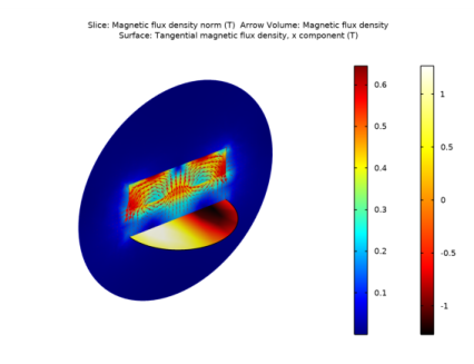
In the Settings window for Surface, click Replace Expression in the upper-right corner of the Expression section. From the menu, choose Component 1 (comp1)>Magnetic Fields, No Currents>Magnetic>Tangential magnetic flux density - T>mfnc.tBx - Tangential magnetic flux density, x component.
3
Locate the Coloring and Style section. From the Color table list, choose Thermal.
4
In the 3D Plot Group 1 toolbar, click  Plot.
To evaluate the force on the plate, integrate the surface stress tensor. Since the plate is modeled by a boundary, the integral must be carried on the two sides of the plates only.
All surfaces have an up and a down side. The physics interface defines variables for the surface stress tensor on the up and downside of the boundaries, for example, mfnc.unTmz and mfnc.dnTmz for the z-component of the magnetic surface stress tensor. To integrate the stress tensor on both sides of the plate it is sufficient to integrate the sum of the two quantities on the boundary.
Surface Integration 1
1
In the Results toolbar, click  More Derived Values and choose Integration>Surface Integration.
2
In the Settings window for Surface Integration, locate the Selection section.
3
From the Selection list, choose Plate.
4
Locate the Expressions section. In the table, enter the following settings:
Here, mfnc.unTmz is the z-component of the Maxwell upward magnetic surface stress tensor, whereas mfnc.dnTmz is the downward equivalent.
5
Click  Evaluate.
Table
1
Go to the Table window.
The result should be 1.3 N. As a comparison, setting k to 0 and solving the model again gives the result 0.40 N. The one-sidedness of the magnet increases the force by approximately a factor 3.
This concludes the part of the application using a linear mu-metal. The remaining instructions show how to use a nonlinear mu-metal.
Modeling Instructions — Nonlinear Mu-Metal
Add Material
1
In the Home toolbar, click  Add Material to open the Add Material window.
2
Go to the Add Material window.
3
In the tree, select Nonlinear Magnetic>Nickel Steel>Nickel Steel Mumetal 77% Ni.
4
Click  Add to Component 1 (comp1).
5
In the Home toolbar, click  Add Material to close the Add Material window.
Materials
Nickel Steel Mumetal 77% Ni (mat3)
1
In the Settings window for Material, locate the Geometric Entity Selection section.
2
From the Geometric entity level list, choose Boundary.
3
From the Selection list, choose Plate.
Magnetic Fields, No Currents (mfnc)
Magnetic Shielding 1
1
In the Model Builder window, under Component 1 (comp1)>Magnetic Fields, No Currents (mfnc) click Magnetic Shielding 1.
2
In the Settings window for Magnetic Shielding, locate the Magnetic Shielding section.
3
From the Magnetization model list, choose B-H curve.
Since the chosen B-H curve is rather steep from a numerical viewpoint, the model may become unstable. The strong nonlinearity in the plate may lead to an abrupt spatial variation of the differential permeability, that is, the ratio dB/dH. For models such as this, it is therefore good practice to switch to linear elements. Switching to linear elements will reduce the model’s ability to resolve the field shape though, you can compensate for this by refining the mesh.
4
In the Model Builder window, click Magnetic Fields, No Currents (mfnc).
5
In the Settings window for Magnetic Fields, No Currents, click to expand the Discretization section.
6
From the Magnetic scalar potential list, choose Linear.
Mesh 1
1
In the Model Builder window, under Component 1 (comp1) click Mesh 1.
2
In the Settings window for Mesh, locate the Mesh Settings section.
3
From the Sequence type list, choose User-controlled mesh.
Size
1
In the Model Builder window, under Component 1 (comp1)>Mesh 1 click Size.
2
In the Settings window for Size, locate the Element Size section.
3
From the Predefined list, choose Finer.
Size 1
1
In the Model Builder window, right-click Free Tetrahedral 1 and choose Size.
2
In the Settings window for Size, locate the Geometric Entity Selection section.
3
From the Geometric entity level list, choose Boundary.
4
From the Selection list, choose Plate.
5
Locate the Element Size section. From the Predefined list, choose Extremely fine.
6
Click  Build All.
7
Click the  Zoom Extents button in the Graphics toolbar.
The mesh should be refined close to the plate. Let us investigate the mesh by creating a plot.
8
In the Mesh toolbar, click  Plot.
Results
Mesh 1
1
In the Settings window for Mesh, locate the Level section.
2
From the Level list, choose All.
3
Locate the Coloring and Style section. From the Element color list, choose Size.
4
From the Color table list, choose Rainbow.
5
Click to expand the Element Filter section. Select the Enable filter check box.
6
In the Expression text field, type y>0.
7
In the Mesh Plot 2 toolbar, click  Plot.
8
Click the  Zoom In button in the Graphics toolbar.
Next, compute the solution. For nonlinear models, the default tolerance of 0.001 may be insufficient, leading to a solution that is not fully converged. Adjust it to improve accuracy.
Study 1
Solver Configurations
In the Model Builder window, expand the Study 1>Solver Configurations node.
Solution 1 (sol1)
1
In the Model Builder window, expand the Study 1>Solver Configurations>Solution 1 (sol1) node, then click Stationary Solver 1.
2
In the Settings window for Stationary Solver, locate the General section.
3
In the Relative tolerance text field, type 1e-4.
4
Click  Compute.
Results
3D Plot Group 1
The nonlinear permeability results in a lower field strength in the plate. To study how far the material is brought into saturation, you can plot the differential permeability (the ratio dB/dH).
Surface 1
1
In the Model Builder window, click Surface 1.
2
In the Settings window for Surface, locate the Expression section.
3
In the Expression text field, type d(comp1.mat3.BHCurve.BH(mfnc.normtH),mfnc.normtH)/mu0_const.
Here, comp1.mat3.BHCurve.BHCurve1() refers to the nonlinear magnetic curve for material 3. Since the operator d(y,x) performs the derivative of y with respect to x, we are plotting the differential relative permeability. A value close to 1 indicates that the material is saturated.
4
In the 3D Plot Group 1 toolbar, click  Plot.
5
In the Results toolbar, click  Evaluate and choose Evaluate All.
Table
1
Go to the Table window.
The result should be around 1.1 N.