PDF

Magnetic Lens
Introduction
Scanning electron microscopes take images of samples by scanning with a high-energy beam of electrons. The subsequent electron interactions produce signals such as secondary and back-scattered electrons that contain information about the sample surface topography. Electromagnetic lenses are used to focus this electron beam down to a spot about 10 nm wide on the sample surface.
Note: This application requires the AC/DC Module and the Particle Tracing Module.
Model Definition
Particles (electrons) are released from near the bottom boundary of the simulation space and pass through a collimator. This collimator can typically be adjusted to remove stray electrons. A simple DC coil produces an axial magnetic field. This rotationally symmetric, inhomogeneous magnetic field results in non-axial electrons experiencing a radial force causing them to spiral about the axis. As they begin to spiral, they have a larger velocity component perpendicular to the mainly axial magnetic field, therefore the radius of their spiral/helical path decreases. Thus, a parallel beam of electrons entering the lens converges to a point.
If the region in which the magnetic field acts upon the electrons is sufficiently small, this coil acts as a ‘thin’ convex lens and the thin lens expression holds.
model equations
A simple model is set up to test the magnetic force within the Charged Particle Tracing interface. The equations solved are the equation of motion of a charged particle in a magnetic field (Lorentz force):
where q (SI unit: C) is the particle charge, v (SI unit: m/s) is the particle velocity, and B (SI unit: T) is the magnetic flux density. The total work done on a particle by a magnetic field is zero.
Results and Discussion
The magnetic flux density is plotted in Figure 1. The strength of the lens depends upon the coil configuration and current. The lenses within electron microscopes are generally very strong, in some cases focusing the electron beam within the lens itself.
Figure 1: Plot of the magnetic flux density in the magnetic lens.
Figure 2 plots the electron trajectories as they travel through the coil. The electrons are focused at a point along the z-axis. The focal length is given by:
where K is a constant based on the coil geometry and number of turns, V is the accelerating voltage and i is the coil current. The focal length increases with electron energy (that is, V) because their high velocity means they spend less time experiencing a force due the magnetic field. However, as the current increases so does the magnetic field strength, therefore the electrons spiral in tighter paths bringing the focal length closer.
Figure 2: Plot of the electron trajectories traveling through the magnetic lens.
When charged particle beams are released, additional global variables are used to define beam properties such as the emittance and the Twiss parameters. These global variables can be used to characterize the shape of a beam and the transverse phase space distribution of the beam particles. In Figure 3 the hyperemittance is plotted along the average beam trajectory as a color expression and as a tube radius expression. The nominal trajectory reaches maximum thickness shortly after entering the lens and appears to be pinched off at the location where the beam is focused.
The ability to change the focal length of a lens is useful as it allows the focusing onto a surface in addition to adjusting the magnification. The effect of the focusing can be seen in Figure 4 which shows a Poincaré map of the particle position at three different snapshots in time. The sharpness of the cross-over can be improved using multiple lenses.
Figure 3: The nominal beam trajectory is plotted, with a color and thickness proportional to the 1-rms hyperemittance of the beam...
Figure 4: Poincaré maps of the particle location in the xy-plane initially (red), at the focal point of the lens (blue), and at the last time step (black).
Reference
1. M.J. Pritchard, Manipulation of Ultracold Atoms Using Magnetic and Optical Fields, PhD thesis, Durham University, September 2006, http://massey.dur.ac.uk/resources/mjpritchard/thesis_pritchard.pdf.
Application Library path: ACDC_Module/Particle_Tracing/magnetic_lens
Modeling Instructions
From the File menu, choose New.
New
In the New window, click  Model Wizard.
Model Wizard
1
In the Model Wizard window, click  3D.
2
In the Select Physics tree, select AC/DC>Electromagnetic Fields>Magnetic Fields (mf).
3
Click Add.
4
Click  Study.
5
In the Select Study tree, select General Studies>Stationary.
6
Global Definitions
Parameters 1
1
In the Model Builder window, under Global Definitions click Parameters 1.
2
In the Settings window for Parameters, locate the Parameters section.
3
Geometry 1
The coil geometry is constructed using cylinders, and it is available as a separate file in the Application Library. Insert the prepared geometry sequence from the file. You can read the instructions for creating the geometry in the appendix.
1
In the Geometry toolbar, click  Insert Sequence.
2
Materials
Material 1 (mat1)
1
In the Model Builder window, under Component 1 (comp1) right-click Materials and choose Blank Material.
2
In the Settings window for Material, locate the Material Contents section.
3
Material 2 (mat2)
1
Right-click Materials and choose Blank Material.
2
3
In the Settings window for Material, locate the Material Contents section.
4
Magnetic Fields (mf)
Coil 1
1
In the Model Builder window, under Component 1 (comp1) right-click Magnetic Fields (mf) and choose the domain setting Coil.
2
3
In the Settings window for Coil, locate the Coil section.
4
From the Conductor model list, choose Homogenized multiturn.
5
From the Coil type list, choose Circular.
6
Locate the Homogenized Multiturn Conductor section. In the N text field, type Nc.
7
Locate the Coil section. In the Icoil text field, type Ic.
Specify the reference edges to be used in the calculation of the current path for the circular coil. To obtain the best results, the selected edges should have a radius close to the average coil radius. In this case, select the edges created for this purpose in previous steps.
Coil Geometry 1
1
In the Model Builder window, click Coil Geometry 1.
2
In the Settings window for Coil Geometry, locate the Edge Selection section.
3
Click  Clear Selection.
4
Mesh 1
Scale 1
1
In the Mesh toolbar, click  Modify and choose Mesh>Scale.
2
In the Settings window for Scale, locate the Geometric Entity Selection section.
3
From the Geometric entity level list, choose Domain.
4
5
Locate the Scale section. In the Element size scale text field, type 0.5.
Free Triangular 1
1
In the Mesh toolbar, click  Boundary and choose Free Triangular.
2
Size 1
1
Right-click Free Triangular 1 and choose Size.
Use a fine mesh on the surface where particles will be released.
2
In the Settings window for Size, locate the Element Size section.
3
From the Predefined list, choose Extremely fine.
Free Tetrahedral 1
1
In the Mesh toolbar, click  Free Tetrahedral.
2
In the Settings window for Free Tetrahedral, click  Build All.
Study 1
In the Home toolbar, click  Compute.
Results
Cut Plane 1
1
In the Model Builder window, expand the Results>Datasets node, then click Cut Plane 1.
2
In the Settings window for Cut Plane, locate the Plane Data section.
3
In the z-coordinate text field, type 0.
Multislice 1
1
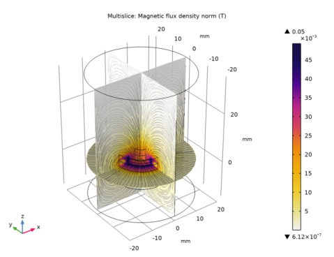
In the Model Builder window, expand the Results>Magnetic Flux Density Norm (mf) node, then click Multislice 1.
2
In the Settings window for Multislice, locate the Multiplane Data section.
3
Find the z-planes subsection. In the Coordinates text field, type 0.
4
Click the  Zoom Extents button in the Graphics toolbar.
5
In the Magnetic Flux Density Norm (mf) toolbar, click  Plot. Compare the resulting image to Figure 1.
Add Physics
1
In the Home toolbar, click  Add Physics to open the Add Physics window.
2
Go to the Add Physics window.
3
In the tree, select AC/DC>Particle Tracing>Charged Particle Tracing (cpt).
4
Find the Physics interfaces in study subsection. In the table, clear the Solve check box for Study 1.
5
Click Add to Component 1 in the window toolbar.
6
In the Home toolbar, click  Add Physics to close the Add Physics window.
Add Study
1
In the Home toolbar, click  Add Study to open the Add Study window.
2
Go to the Add Study window.
3
Find the Studies subsection. In the Select Study tree, select General Studies>Time Dependent.
4
Find the Physics interfaces in study subsection. In the table, clear the Solve check box for Magnetic Fields (mf).
5
Click Add Study in the window toolbar.
6
In the Home toolbar, click  Add Study to close the Add Study window.
Geometry 1
In the Model Builder window, collapse the Component 1 (comp1)>Geometry 1 node.
Charged Particle Tracing (cpt)
1
In the Model Builder window, under Component 1 (comp1) click Charged Particle Tracing (cpt).
2
In the Settings window for Charged Particle Tracing, locate the Domain Selection section.
3
Click  Clear Selection.
4
Particle Properties 1
1
In the Model Builder window, under Component 1 (comp1)>Charged Particle Tracing (cpt) click Particle Properties 1.
2
In the Settings window for Particle Properties, locate the Particle Species section.
3
From the Particle species list, choose Electron.
You need to provide the forces acting on the particles; in this case, the magnetic (Lorentz) force.
Magnetic Force 1
1
In the Physics toolbar, click  Domains and choose Magnetic Force.
2
3
In the Settings window for Magnetic Force, locate the Magnetic Force section.
4
From the B list, choose Magnetic flux density (mf).
Particle Beam 1
1
In the Physics toolbar, click  Boundaries and choose Particle Beam.
2
3
In the Settings window for Particle Beam, locate the Initial Position section.
4
In the N text field, type 10000.
5
Locate the Initial Transverse Velocity section. In the εrms text field, type 0.1[um].
6
Locate the Initial Longitudinal Velocity section. In the E text field, type 0.5[keV].
Study 2
Step 1: Time Dependent
1
In the Model Builder window, under Study 2 click Step 1: Time Dependent.
2
In the Settings window for Time Dependent, click to expand the Values of Dependent Variables section.
3
Find the Values of variables not solved for subsection. From the Settings list, choose User controlled.
4
From the Method list, choose Solution.
5
From the Study list, choose Study 1, Stationary.
6
Locate the Study Settings section. Click  Range.
7
In the Range dialog box, choose Number of values from the Entry method list.
8
In the Stop text field, type 5e-9.
9
In the Number of values text field, type 50.
10
Click Replace.
11
In the Home toolbar, click  Compute.
Results
Particle Trajectories (cpt)
In the Model Builder window, expand the Particle Trajectories (cpt) node.
Particle Trajectories 1
1
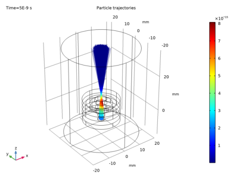
In the Model Builder window, expand the Results>Particle Trajectories (cpt)>Particle Trajectories 1 node, then click Particle Trajectories 1.
2
In the Settings window for Particle Trajectories, locate the Coloring and Style section.
3
Find the Line style subsection. From the Type list, choose Line.
4
Find the Point style subsection. From the Type list, choose None.
Color Expression 1
1
In the Model Builder window, click Color Expression 1.
2
In the Settings window for Color Expression, locate the Expression section.
3
In the Expression text field, type sqrt(cpt.Ftx^2+cpt.Fty^2+cpt.Ftz^2).
4
In the Particle Trajectories (cpt) toolbar, click  Plot.
5
Click the  Zoom Extents button in the Graphics toolbar. Compare the resulting image to Figure 2.
Now observe the beam hyperemittance along the nominal beam trajectory.
Average Beam Position and Hyperemittance
1
In the Model Builder window, under Results click Average Beam Position (cpt).
2
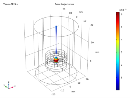
In the Settings window for 3D Plot Group, type Average Beam Position and Hyperemittance in the Label text field.
Point Trajectories 1
1
In the Model Builder window, expand the Average Beam Position and Hyperemittance node, then click Point Trajectories 1.
2
In the Settings window for Point Trajectories, locate the Coloring and Style section.
3
Find the Line style subsection. From the Type list, choose Tube.
4
Click  Replace Expression.
5
From the menu, choose Component 1 (comp1)>Charged Particle Tracing>Beam properties>cpt.e1hrms - 1-RMS beam hyperemittance - .
6
Select the Radius scale factor check box.
7
8
From the Interpolation list, choose Uniform.
9
In the Average Beam Position and Hyperemittance toolbar, click  Plot. Compare the resulting image to Figure 3.
Now construct a Poincaré Map to visualize the radial distribution of particles initially, at the focal point, and at the exit of the modeling domain.
Cut Plane 4
1
In the Results toolbar, click  Cut Plane.
2
In the Settings window for Cut Plane, locate the Plane Data section.
3
From the Plane list, choose xy-planes.
4
In the z-coordinate text field, type -6.
5
Locate the Data section. From the Dataset list, choose Particle 1.
Cut Plane 5
1
Right-click Cut Plane 4 and choose Duplicate.
2
In the Settings window for Cut Plane, locate the Plane Data section.
3
In the z-coordinate text field, type 7.
Cut Plane 6
1
Right-click Cut Plane 5 and choose Duplicate.
2
In the Settings window for Cut Plane, locate the Plane Data section.
3
In the z-coordinate text field, type 34.
Poincaré Maps
1
In the Results toolbar, click  2D Plot Group.
2
In the Settings window for 2D Plot Group, type Poincaré Maps in the Label text field.
3
Locate the Data section. From the Dataset list, choose Particle 1.
4
Click to expand the Title section. From the Title type list, choose Manual.
5
In the Title text area, type Poincaré Map.
Poincaré Map 1
1
In the Poincaré Maps toolbar, click  More Plots and choose Poincaré Map.
2
In the Settings window for Poincaré Map, locate the Data section.
3
From the Cut plane list, choose Cut Plane 6.
4
Locate the Coloring and Style section. From the Color list, choose Black.
5
Click the  Zoom Extents button in the Graphics toolbar.
Poincaré Map 2
1
Right-click Poincaré Map 1 and choose Duplicate.
2
In the Settings window for Poincaré Map, locate the Data section.
3
From the Cut plane list, choose Cut Plane 4.
4
Locate the Coloring and Style section. From the Color list, choose Red.
Poincaré Map 3
1
Right-click Poincaré Map 2 and choose Duplicate.
2
In the Settings window for Poincaré Map, locate the Data section.
3
From the Cut plane list, choose Cut Plane 5.
4
Locate the Coloring and Style section. From the Color list, choose Blue.
5
In the Poincaré Maps toolbar, click  Plot.
6
Click the  Zoom Extents button in the Graphics toolbar. Compare the resulting image to Figure 4.
 
Appendix A - Geometry Instructions
Add Component
In the Home toolbar, click  Add Component and choose 3D.
Geometry 1
1
In the Settings window for Geometry, locate the Units section.
2
From the Length unit list, choose mm.
Cylinder 1 (cyl1)
1
In the Geometry toolbar, click  Cylinder.
2
In the Settings window for Cylinder, locate the Size and Shape section.
3
In the Radius text field, type 10.
4
In the Height text field, type 2.5.
Cylinder 2 (cyl2)
1
In the Geometry toolbar, click  Cylinder.
2
In the Settings window for Cylinder, locate the Size and Shape section.
3
In the Radius text field, type 6.
4
In the Height text field, type 2.5.
5
Click  Build Selected.
Cylinder 3 (cyl3)
1
In the Model Builder window, under Component 1 (comp1)>Geometry 1 right-click Cylinder 1 (cyl1) and choose Duplicate.
2
In the Settings window for Cylinder, locate the Position section.
3
In the z text field, type -7.5.
Cylinder 4 (cyl4)
1
In the Geometry toolbar, click  Cylinder.
2
In the Settings window for Cylinder, locate the Size and Shape section.
3
In the Radius text field, type 2.
4
In the Height text field, type 2.5.
5
Locate the Position section. In the z text field, type -7.5.
Cylinder 5 (cyl5)
1
Right-click Cylinder 1 (cyl1) and choose Duplicate.
2
In the Settings window for Cylinder, locate the Position section.
3
In the z text field, type -2.5.
Cylinder 6 (cyl6)
1
In the Geometry toolbar, click  Cylinder.
2
In the Settings window for Cylinder, locate the Size and Shape section.
3
In the Radius text field, type 3.
4
In the Height text field, type 2.5.
5
Locate the Position section. In the z text field, type -2.5.
Cylinder 7 (cyl7)
1
Right-click Cylinder 1 (cyl1) and choose Duplicate.
2
In the Settings window for Cylinder, locate the Position section.
3
In the z text field, type 2.5.
Cylinder 8 (cyl8)
1
In the Geometry toolbar, click  Cylinder.
2
In the Settings window for Cylinder, locate the Size and Shape section.
3
In the Radius text field, type 3.
4
In the Height text field, type 2.5.
5
Locate the Position section. In the z text field, type 2.5.
Cylinder 9 (cyl9)
1
In the Geometry toolbar, click  Cylinder.
2
In the Settings window for Cylinder, locate the Size and Shape section.
3
In the Radius text field, type 20.
4
In the Height text field, type 50.
5
Locate the Position section. In the z text field, type -15.
Difference 1 (dif1)
1
In the Geometry toolbar, click  Booleans and Partitions and choose Difference.
2
Select the objects cyl1, cyl3, cyl5, and cyl7 only.
3
In the Settings window for Difference, locate the Difference section.
4
Find the Objects to subtract subsection. Select the  Activate Selection toggle button.
5
Select the objects cyl2, cyl4, cyl6, and cyl8 only.
6
Click  Build Selected.
7
Click the  Go to Default View button in the Graphics toolbar.
Work Plane 1 (wp1)
1
In the Geometry toolbar, click  Work Plane.
2
Click the  Wireframe Rendering button in the Graphics toolbar.
3
In the Settings window for Work Plane, locate the Plane Definition section.
4
From the Plane type list, choose Face parallel.
5
On the object dif1, select Boundary 3 only.
6
Click  Show Work Plane.
Work Plane 1 (wp1)>Plane Geometry
Click the  Zoom Extents button in the Graphics toolbar.
Work Plane 1 (wp1)>Circle 1 (c1)
1
In the Work Plane toolbar, click  Circle.
2
In the Settings window for Circle, locate the Size and Shape section.
3
In the Radius text field, type 2.
4
Click  Build Selected.
Last, create a circular edge to be used in the Coil feature as a reference edge.
Work Plane 2 (wp2)
1
In the Model Builder window, right-click Geometry 1 and choose Work Plane.
2
In the Settings window for Work Plane, locate the Plane Definition section.
3
From the Plane type list, choose Face parallel.
4
On the object dif1, select Boundary 13 only.
5
Click  Show Work Plane.
Work Plane 2 (wp2)>Circle 1 (c1)
1
In the Work Plane toolbar, click  Circle.
2
In the Settings window for Circle, locate the Object Type section.
3
From the Type list, choose Curve.
4
Locate the Size and Shape section. In the Radius text field, type 8.
5
In the Work Plane toolbar, click  Build All.