|
|
|
|
1
|
|
2
|
|
3
|
Click Add.
|
|
4
|
Click
|
|
5
|
|
6
|
Click
|
|
1
|
|
2
|
|
3
|
|
1
|
|
2
|
|
3
|
|
4
|
|
5
|
|
6
|
|
1
|
|
2
|
|
3
|
|
4
|
|
5
|
|
6
|
|
1
|
|
2
|
|
3
|
|
4
|
|
5
|
|
6
|
|
7
|
|
1
|
|
2
|
|
3
|
|
4
|
|
5
|
|
6
|
|
7
|
|
1
|
|
2
|
|
4
|
|
5
|
|
6
|
|
1
|
|
2
|
|
1
|
|
2
|
|
3
|
In the tree, select Built-in>Air.
|
|
4
|
|
5
|
|
6
|
|
7
|
|
1
|
|
2
|
|
3
|
Specify the A vector as
|
|
1
|
|
3
|
|
4
|
|
5
|
Locate the Constitutive Relation Jc-E section. From the σ list, choose User defined. In the associated text field, type 1000.
|
|
1
|
|
3
|
|
4
|
|
5
|
|
6
|
|
7
|
|
8
|
|
9
|
|
1
|
|
2
|
|
3
|
|
4
|
|
1
|
In the Model Builder window, under Component 1 (comp1)>Magnetic Fields (mf) right-click Coil 1 and choose Duplicate.
|
|
2
|
|
3
|
|
4
|
|
1
|
|
2
|
|
3
|
|
4
|
Find the Physics interfaces in study subsection. In the table, clear the Solve check box for Study 1.
|
|
5
|
|
6
|
|
1
|
|
2
|
|
3
|
|
4
|
|
5
|
|
1
|
In the Model Builder window, under Component 1 (comp1) right-click Electrical Circuit (cir) and choose Import SPICE Netlist.
|
|
3
|
|
1
|
|
2
|
|
1
|
|
2
|
|
3
|
|
1
|
|
2
|
|
3
|
|
4
|
In the Physics and variables selection tree, select Component 1 (comp1)>Magnetic Fields (mf)>Coil 2.
|
|
5
|
Click
|
|
6
|
|
7
|
|
1
|
|
2
|
|
3
|
|
4
|
|
5
|
|
6
|
Locate the Physics and Variables Selection section. Select the Modify model configuration for study step check box.
|
|
7
|
In the Physics and variables selection tree, select Component 1 (comp1)>Magnetic Fields (mf)>Coil 1.
|
|
8
|
Click
|
|
1
|
|
2
|
|
3
|
|
4
|
Click
|
|
6
|
Locate the Physics and Variables Selection section. Select the Modify model configuration for study step check box.
|
|
7
|
In the Physics and variables selection tree, select Component 1 (comp1)>Magnetic Fields (mf)>Coil 1.
|
|
8
|
Click
|
|
1
|
|
2
|
|
3
|
|
4
|
|
5
|
|
6
|
|
7
|
|
8
|
|
1
|
In the Model Builder window, under Component 1 (comp1)>Electrical Circuit (cir) click External I vs. U 1 (IvsU1).
|
|
2
|
|
3
|
|
1
|
|
2
|
|
3
|
|
4
|
|
5
|
|
6
|
|
7
|
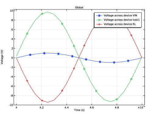
In the associated text field, type Time (s).
|
|
8
|
|
9
|
In the associated text field, type Voltage (V).
|
|
1
|
|
2
|
|
4
|
Click to expand the Coloring and Style section. Find the Line markers subsection. From the Marker list, choose Cycle.
|
|
1
|
|
2
|
|
3
|
Click OK.
|
|
1
|
|
2
|
|
3
|