|
|
|
|
5.998·107 S/m
|
|||
|
εr
|
|||
|
μr
|
103
|
|
1
|
|
2
|
|
3
|
Click Add.
|
|
4
|
|
5
|
Click
|
|
6
|
|
7
|
Click
|
|
1
|
|
2
|
|
3
|
Click Browse.
|
|
4
|
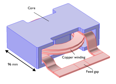
Browse to the model’s Application Libraries folder and double-click the file inductor_3d.mphbin.
|
|
5
|
Click Import.
|
|
1
|
|
2
|
|
3
|
|
4
|
Click to expand the Layers section. In the table, enter the following settings:
|
|
5
|
|
1
|
|
2
|
|
3
|
|
1
|
|
3
|
|
4
|
|
5
|
Click OK.
|
|
1
|
|
3
|
|
4
|
|
5
|
Click OK.
|
|
1
|
|
3
|
|
4
|
|
5
|
Click OK.
|
|
1
|
|
3
|
|
4
|
|
5
|
Click OK.
|
|
1
|
|
3
|
|
4
|
|
5
|
Click OK.
|
|
1
|
|
3
|
|
4
|
|
5
|
Click OK.
|
|
1
|
|
2
|
|
3
|
|
4
|
|
1
|
|
2
|
|
3
|
In the tree, select AC/DC>Copper.
|
|
4
|
|
5
|
In the tree, select Built-in>Air.
|
|
6
|
|
7
|
|
1
|
|
2
|
|
3
|
|
1
|
|
2
|
|
3
|
|
1
|
|
2
|
|
3
|
|
4
|
|
5
|
|
6
|
|
7
|
Click OK.
|
|
1
|
|
2
|
|
3
|
|
4
|
|
1
|
In the Model Builder window, expand the Component 1 (comp1)>Magnetic Fields (mf)>Coil 1>Geometry Analysis 1 node, then click Input 1.
|
|
1
|
|
1
|
|
2
|
|
3
|
|
1
|
|
2
|
|
3
|
|
1
|
|
2
|
|
1
|
|
2
|
|
3
|
|
4
|
|
1
|
|
2
|
|
3
|
|
4
|
|
1
|
|
2
|
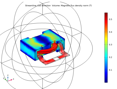
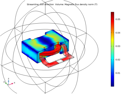
In the Settings window for Streamline, click Replace Expression in the upper-right corner of the Expression section. From the menu, choose Component 1 (comp1)>Magnetic Fields>Coil parameters>mf.coil1.eCoilx,...,mf.coil1.eCoilz - Coil direction.
|
|
1
|
|
2
|
|
3
|
|
4
|
|
5
|
|
6
|
|
1
|
|
2
|
|
4
|
Click
|
|
1
|
Go to the Table window.
|
|
1
|
|
1
|
|
2
|
|
1
|
|
2
|
|
3
|
|
4
|
|
5
|
|
1
|
|
2
|
|
3
|
|
1
|
|
2
|
|
1
|
|
2
|
|
4
|
|
1
|
|
2
|
|
3
|
|
4
|
|
1
|
|
2
|
|
4
|
Click
|
|
1
|
Go to the Table window.
|
|
1
|
|
2
|
|
3
|
Find the Physics interfaces in study subsection. In the table, clear the Solve check box for Electrical Circuit (cir).
|
|
4
|
|
5
|
|
6
|
|
1
|
|
3
|
|
4
|
|
5
|
|
6
|
|
7
|
Click OK.
|
|
1
|
|
2
|
|
3
|
In the tree, select AC/DC>Copper.
|
|
4
|
|
5
|
|
1
|
|
2
|
|
3
|
|
1
|
|
2
|
|
3
|
|
1
|
|
2
|
|
3
|
|
1
|
|
1
|
|
3
|
|
4
|
|
5
|
|
6
|
|
7
|
|
8
|
|
1
|
|
2
|
|
3
|
|
4
|
Locate the Constitutive Relation B-H section. From the Magnetization model list, choose Magnetic losses.
|
|
5
|
From the μ′ list, choose User defined. From the μ′′ list, choose User defined. In the μ′ text field, type 1200.
|
|
6
|
|
1
|
|
2
|
|
3
|
|
4
|
Click
|
|
5
|
|
6
|
|
7
|
|
8
|
Click Replace.
|
|
9
|
|
1
|
|
2
|
|
3
|
|
4
|
|
1
|
|
2
|
|
3
|
|
4
|
|
1
|
|
2
|
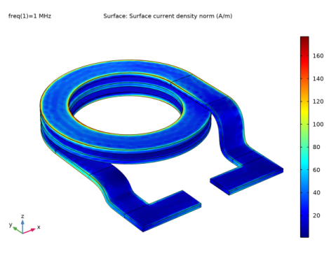
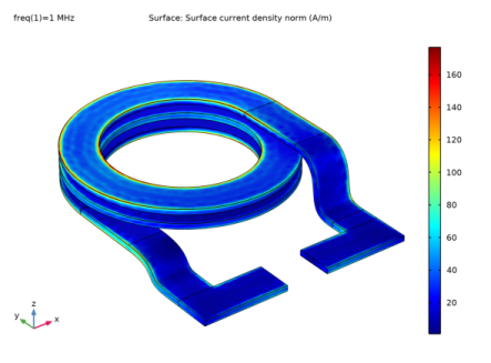
In the Settings window for Surface, click Replace Expression in the upper-right corner of the Expression section. From the menu, choose Component 1 (comp1)>Magnetic Fields>Currents and charge>mf.normJs - Surface current density norm - A/m.
|
|
1
|
|
2
|
|
1
|
|
2
|
|
3
|
|
1
|
|
2
|
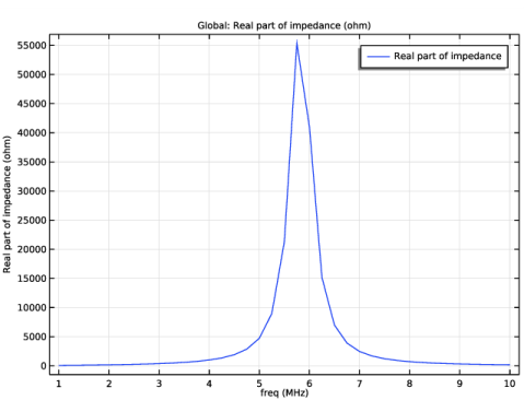
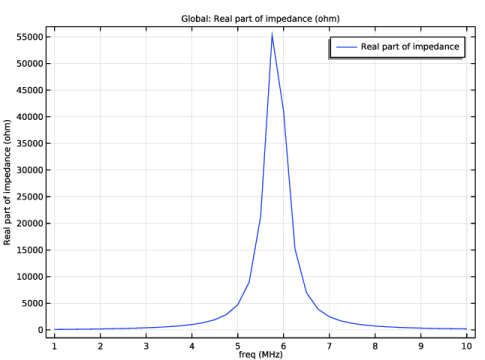
In the Settings window for Global, click Replace Expression in the upper-right corner of the y-Axis Data section. From the menu, choose Component 1 (comp1)>Magnetic Fields>Ports>mf.Zport_1 - Lumped port impedance - Ω.
|
|
3
|
|
4
|
|
5
|
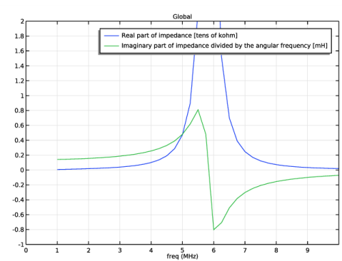
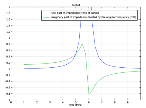
Click Replace Expression in the upper-right corner of the y-Axis Data section. From the menu, choose Component 1 (comp1)>Magnetic Fields>Ports>mf.Zport_1 - Lumped port impedance - Ω.
|
|
6
|
|
1
|
|
2
|
|
3
|
|
4
|
|
5
|
|
6
|
|
7
|
|
8
|