|
|
|
|
1
|
|
2
|
In the Select Physics tree, select AC/DC>Electromagnetic Fields>Vector Formulations>Magnetic and Electric Fields (mef).
|
|
3
|
Click Add.
|
|
4
|
Click
|
|
5
|
|
6
|
Click
|
|
1
|
|
2
|
|
1
|
|
2
|
|
3
|
|
1
|
|
2
|
|
3
|
|
4
|
|
5
|
|
6
|
|
1
|
|
2
|
|
1
|
|
2
|
|
3
|
|
4
|
|
5
|
|
6
|
|
1
|
|
2
|
|
1
|
|
2
|
|
3
|
|
4
|
|
5
|
|
1
|
|
2
|
|
3
|
|
4
|
|
5
|
|
6
|
|
7
|
Click to expand the Layers section. In the table, enter the following settings:
|
|
8
|
|
9
|
|
10
|
|
1
|
|
2
|
|
3
|
|
4
|
|
5
|
|
6
|
|
7
|
|
1
|
In the Model Builder window, under Component 1 (comp1)>Geometry 1 right-click Work Plane 1 (wp1) and choose Extrude.
|
|
2
|
Select the object wp1.r1 only.
|
|
3
|
|
4
|
Locate the Distances section. In the table, enter the following settings:
|
|
1
|
|
2
|
Select the object ext1 only.
|
|
3
|
|
4
|
|
5
|
Select the object cyl3 only.
|
|
6
|
|
1
|
|
2
|
|
3
|
Locate the Distances section. In the table, enter the following settings:
|
|
1
|
|
2
|
|
3
|
|
4
|
|
5
|
|
6
|
|
1
|
|
2
|
|
3
|
|
4
|
|
5
|
|
6
|
|
7
|
|
1
|
In the Model Builder window, under Component 1 (comp1)>Geometry 1 right-click Work Plane 2 (wp2) and choose Extrude.
|
|
2
|
|
3
|
Locate the Distances section. In the table, enter the following settings:
|
|
1
|
|
2
|
Select the object ext3 only.
|
|
3
|
|
4
|
|
5
|
Select the object cyl1 only.
|
|
6
|
|
1
|
|
2
|
|
3
|
|
4
|
|
5
|
|
6
|
|
1
|
|
2
|
|
3
|
|
1
|
|
2
|
|
3
|
|
4
|
|
1
|
|
2
|
|
3
|
|
4
|
|
5
|
|
6
|
Click OK.
|
|
7
|
|
8
|
|
9
|
Click OK.
|
|
1
|
|
3
|
|
4
|
|
5
|
Click OK.
|
|
1
|
|
2
|
|
3
|
|
4
|
|
5
|
Click OK.
|
|
6
|
|
7
|
|
8
|
Click OK.
|
|
1
|
In the Model Builder window, under Component 1 (comp1) right-click Magnetic and Electric Fields (mef) and choose Ampère’s Law.
|
|
1
|
|
2
|
|
3
|
|
4
|
|
1
|
|
2
|
|
3
|
|
4
|
|
1
|
|
2
|
|
3
|
In the tree, select Built-in>Air.
|
|
4
|
|
5
|
In the tree, select AC/DC>Copper.
|
|
6
|
|
7
|
|
1
|
|
2
|
|
1
|
|
2
|
|
1
|
|
2
|
|
3
|
|
4
|
|
5
|
|
6
|
|
1
|
|
2
|
|
1
|
|
2
|
|
3
|
|
4
|
|
1
|
|
2
|
|
1
|
|
2
|
|
3
|
|
4
|
|
1
|
|
2
|
|
3
|
|
1
|
|
2
|
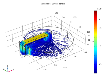
In the Settings window for Streamline, click Replace Expression in the upper-right corner of the Expression section. From the menu, choose Component 1 (comp1)>Magnetic and Electric Fields>Currents and charge>mef.Jx,mef.Jy,mef.Jz - Current density.
|
|
3
|
|
4
|
|
5
|
|
6
|
Click OK.
|
|
7
|
|
8
|
|
9
|
|
1
|
|
2
|
|
3
|
|
4
|
|
1
|
|
2
|
|
3
|
Click OK.
|
|
4
|
|
1
|
|
2
|
|
3
|
|
1
|
|
2
|
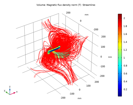
In the Settings window for Volume, click Replace Expression in the upper-right corner of the Expression section. From the menu, choose Component 1 (comp1)>Magnetic and Electric Fields>Magnetic>mef.normB - Magnetic flux density norm - T.
|
|
3
|
|
4
|
|
5
|
Click OK.
|
|
1
|
|
2
|
|
3
|
|
4
|
|
5
|
|
6
|
|
7
|
|
8
|
Click OK.
|
|
9
|
|
10
|
|
11
|
|
12
|
Click OK.
|
|
1
|
|
2
|
|
3
|
Click OK.
|
|
1
|
|
2
|
|
3
|
|
1
|
|
2
|
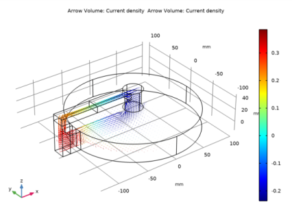
In the Settings window for Arrow Volume, click Replace Expression in the upper-right corner of the Expression section. From the menu, choose Component 1 (comp1)>Magnetic and Electric Fields>Currents and charge>mef.Jx,mef.Jy,mef.Jz - Current density.
|
|
3
|
Locate the Arrow Positioning section. Find the x grid points subsection. In the Points text field, type 40.
|
|
4
|
|
5
|
|
6
|
|
7
|
|
1
|
|
2
|
|
1
|
In the Model Builder window, under Results>3D Plot Group 3 right-click Arrow Volume 1 and choose Duplicate.
|
|
2
|
In the Settings window for Arrow Volume, click Replace Expression in the upper-right corner of the Expression section. From the menu, choose Component 1 (comp1)>Magnetic and Electric Fields>Currents and charge>mef.Jx,mef.Jy,mef.Jz - Current density.
|
|
3
|
Locate the Arrow Positioning section. Find the x grid points subsection. In the Points text field, type 80.
|
|
4
|
|
5
|
|
6
|
|
7
|
|
8
|
|
1
|
|
2
|
|
3
|
|
1
|
|
2
|
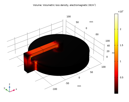
In the Settings window for Volume, click Replace Expression in the upper-right corner of the Expression section. From the menu, choose Component 1 (comp1)>Magnetic and Electric Fields>Heating and losses>mef.Qh - Volumetric loss density, electromagnetic - W/m³.
|
|
3
|
|
4
|
|
1
|
|
3
|
In the Settings window for Surface Integration, click Replace Expression in the upper-right corner of the Expressions section. From the menu, choose Component 1 (comp1)>Magnetic and Electric Fields>Currents and charge>mef.normJ - Current density norm - A/m².
|
|
4
|
Click
|
|
1
|
Go to the Table window.
|