|
|
|
|
1
|
|
2
|
In the Select Physics tree, select AC/DC>Electric Fields and Currents>Electrostatics, Boundary Elements (esbe).
|
|
3
|
Click Add.
|
|
4
|
Click
|
|
5
|
|
6
|
Click
|
|
1
|
|
2
|
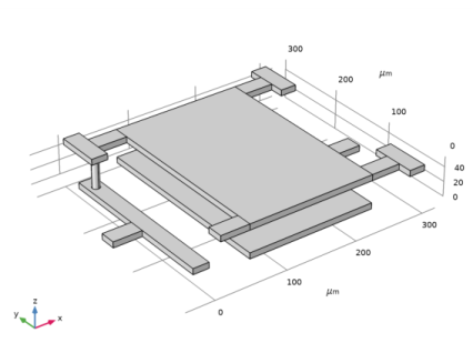
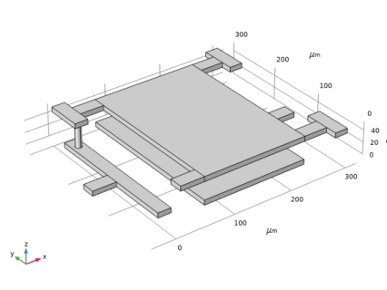
Browse to the model’s Application Libraries folder and double-click the file capacitor_tunable_geom_sequence.mph.
|
|
3
|
|
4
|
|
1
|
|
2
|
|
4
|
|
1
|
|
2
|
|
4
|
|
1
|
In the Model Builder window, under Component 1 (comp1) right-click Materials and choose Blank Material.
|
|
2
|
|
3
|
|
4
|
|
1
|
In the Model Builder window, under Component 1 (comp1) click Electrostatics, Boundary Elements (esbe).
|
|
2
|
|
3
|
|
1
|
|
2
|
|
3
|
|
1
|
|
2
|
|
3
|
|
4
|
|
1
|
|
2
|
|
3
|
|
4
|
|
1
|
|
2
|
|
3
|
In the Model Builder window, expand the Study 1>Solver Configurations>Solution 1 (sol1)>Stationary Solver 1 node.
|
|
4
|
Right-click Study 1>Solver Configurations>Solution 1 (sol1)>Stationary Solver 1>Suggested Direct Solver (esbe) and choose Enable.
|
|
5
|
|
1
|
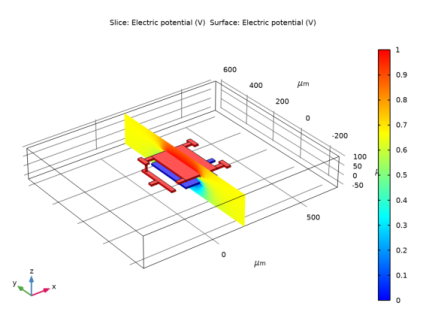
In the Model Builder window, expand the Electric Potential, Domains (esbe) node, then click Surface 1.
|
|
2
|
|
3
|
|
1
|
|
2
|
|
3
|
|
4
|
|
5
|
|
6
|
|
7
|
|
8
|
|
9
|
|
10
|
|
1
|
|
2
|
|
3
|
|
4
|
|
5
|
|
6
|
|
7
|
|
8
|
|
10
|
|
11
|
|
12
|
|
1
|
|
2
|
In the Settings window for Global Evaluation, click Replace Expression in the upper-right corner of the Expressions section. From the menu, choose Component 1 (comp1)>Electrostatics, Boundary Elements>Terminals>esbe.C11 - Maxwell capacitance - F.
|
|
3
|
Locate the Expressions section. In the table, enter the following settings:
|
|
4
|
Click
|
|
1
|
Go to the Table window.
|