The Physics Interface Syntax

Create a physics interface instance using the syntax:

phys = comp.physics.create(<phystag>, physint, <geomtag>)

where <phystag> is a string that identifies the physics interface node. Once defined, you can always refer to a physics interface, or any other feature, by its tag. The string physint is the constructor name of the physics interface. To get the constructor name, the best way is to create a model using the desired physics interface in the GUI and save the model as an M-file. The string <geomtag> refers to the geometry where you want to specify the interface.

To add a feature to a physics interface, use the syntax:

phys.feature.create(<ftag>, operation)

where <ftag> is a string that you use to refer to the operation. To set a property to a value in a operation, enter:

phys.feature(<ftag>).set(property, <value>)

where <ftag> is the string that identifies the feature.


	There are alternative syntaxes available. See model.physics() in the COMSOL Multiphysics Programming Reference Manual or type at the MATLAB prompt: mphdoc(model.physics).

To disable or remove a feature node, use the methods active or remove, respectively.

The command:

phys.feature(<ftag>).active(false)

disables the feature <ftag>.

To activate the feature node you can set the active method to true:

phys.feature(<ftag>).active(true)

To remove a feature from the model, use the method remove:

phys.feature.remove(<ftag>)

Example: Implement and Solve a Heat Transfer Problem

This example shows how to add a physics interface and set the boundary conditions in the model object.

Start to create a model object including a 3D geometry. The geometry consists in a block with default settings. Enter the following commands at the MATLAB prompt:

model = ModelUtil.create('Model');

comp1 = model.component.create('comp1', true);

geom1 = comp1.geom.create('geom1', 3);

geom1.feature.create('blk1', 'Block');

geom1.run;

Add a Heat Transfer in Solids interface to the model:

phys = comp1.physics.create('ht', 'HeatTransfer', 'geom1');

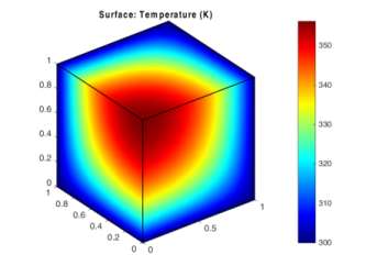
The tag of the interface is ht. The interface constructor is HeatTransfer. The physics is defined on geometry geom1.

The physics interface automatically creates a number of default features. To examine these, enter:

comp1.physics('ht')

ans =

Type: Heat Transfer in Solids

Tag: ht

Identifier: ht

Operation: HeatTransfer

Child nodes: solid1, init1, ins1, idi1, os1, cib1

The physics method has the following child nodes: solid1, init1, ins1, idi1, os1, and cib1. These are the default features that come with the Heat Transfer in Solids interface. The first feature, solid1, consists of the heat balance equation. Confirm this by entering:

solid = phys.feature('solid1')

ans =

Type: Solid

Tag: solid1

Operation: SolidHeatTransferModel

The settings of the solid1 feature node can be modified, for example, to manually set the material property. To change the thermal conductivity to 400 W/(m*K) enter:

solid.set('k_mat', 1, 'userdef');

solid.set('k', 400);

The Heat Transfer in Solids interface has features you can use to specify domain or boundary settings. For example, to add a heat source of 105 W/m3 in the study domain, enter the commands:

hs = phys.feature.create('hs1', 'HeatSource', 3);

hs.selection.set(1);

hs.set('Q', 1, 1e5);

To create a temperature boundary condition on boundaries 3, 5, and 6, enter:

temp = phys.feature.create('temp1', 'TemperatureBoundary', 2);

temp.selection.set([3 5 6]);

temp.set('T0', 1, '300[K]');

Then add a mesh and a study feature and compute the solution:

comp1.mesh.create('mesh1');