Mesh Creation Functions

The Size attribute provides a number of input properties that can control the mesh element size, such as the following properties:

These properties are available both globally and locally. The following examples are included: Creating a 2D Mesh with Triangular Elements and Creating a 2D Mesh with Quadrilateral Elements. Also discussed is The Free Meshing Method.

There are several predefined settings that can be used to set a suitable combination of values for many properties. To select one of these settings, use the property hauto and pass an integer from 1 to 9 as its value to describe the mesh resolution:

	For details about predefined mesh size settings and mesh element size parameters, see Size in the COMSOL Multiphysics Programming Reference Manual.

Generate a triangular mesh of a unit square:

The default size feature is generated with the property hauto set to 5, that is:

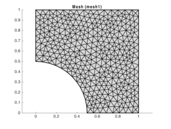
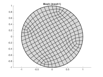
To override this behavior, set hauto to another integer. Override this by setting specific size properties, for example, making the mesh finer than the default by specifying a maximum element size of 0.02:

This value corresponds to 1/50 of the largest axis-parallel distance, whereas the default value is 1/15.

Sometimes a nonuniform mesh is desirable. Make a mesh that is denser on the left side by specifying a smaller maximum element size only on the edge segment to the left (edge number 1):

The default method to generate free triangle meshes in 2D is based on an advancing front algorithm. To switch to a Delaunay algorithm use the value del for the method property. Start by creating a geometry:

To create an unstructured quadrilateral mesh on a unit circle, enter:

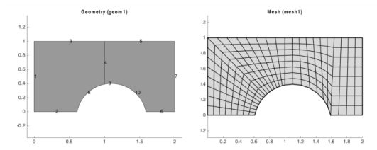
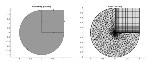
To create a structured quadrilateral mesh in 2D, use the Map operation. This operation uses a mapping technique to create the quadrilateral mesh.

	Map in the COMSOL Multiphysics Programming Reference Manual

Use the EdgeGroup attribute to group the edges (boundaries) into four edge groups, one for each edge of the logical mesh. To control the edge element distribution use the Distribution attribute, which determines the overall mesh density.

Create a structured quadrilateral mesh on a geometry where the domains are bounded by more than four edges:

The left-hand side plot in Figure 3-6 is obtained with this command:

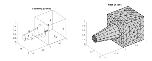
The EdgeGroup attributes specify that the four edges enclosing domain 1 are boundaries 1 and 3; boundary 2; boundary 8; and boundary 4. For domain 2 the four edges are boundary 4; boundary 5; boundary 7; and boundaries 9, 10, and 6.

To build meshes in a step-by-step fashion, create selections for the parts of the geometry that you want to mesh in each step, as in this example:

The final mesh is in Figure 3-7. Note the effect of the Distribution feature, with which the distribution of vertex elements along geometry edges can be controlled.

The left-hand side plot in Figure 3-7 is obtained with this command:

To replace the structured quad mesh by an unstructured quad mesh, delete the Map feature and replace it by a FreeQuad feature:

	Analogous to working with the meshing sequence in the Model Builder in the COMSOL Desktop, new features are always inserted after the current feature.

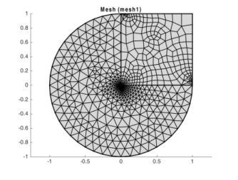
Thus, to get the FreeQuad feature before the FreeTri feature, the dis1 feature needs to be made the current feature by building it with the run method. Alternatively, parts of a mesh can be selectively removed by using the Delete feature. For example, to remove the structured mesh from domain 2 (along with the adjacent edge mesh on edges 3 and 4), and replace it with an unstructured quad mesh, enter these commands:

	For further details on the various commands and their properties see the COMSOL Multiphysics Programming Reference Manual.

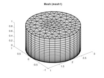
Create 3D volume meshes by extruding and revolving face meshes with the Sweep feature. Depending on the 2D mesh type, the 3D meshes can be hexahedral (brick) meshes or prism meshes.

Create and visualize a revolved prism mesh as follows:

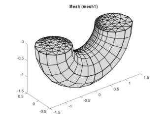
To obtain a torus, leave the angles property unspecified; the default value gives a complete revolution.

To generate a 3D prism mesh from the same 2D mesh by extrusion and then to plot it, enter these commands:

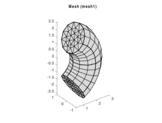
The result is shown in Figure 3-9. With the properties elemcount and elemratio the number and distribution of mesh element layers is controlled in the extruded direction.

	Distribution in the COMSOL Multiphysics Programming Reference Manual or at the MATLAB prompt: mphdoc(model.mesh,'Distribution')

By specifying selections for the meshing operations, swept meshing can also be combined with free meshing. In this case, start by free meshing domain 2, then sweep the resulting surface mesh through domain 1, as in this example:

The left-hand side plot in Figure 3-10 is obtained with this command:

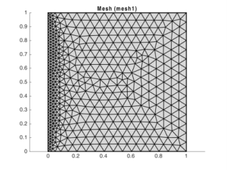
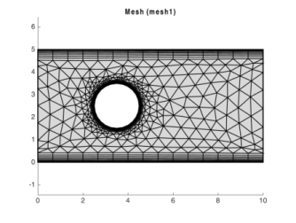
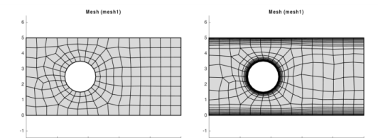
For 2D and 3D geometries it is also possible to create boundary layer meshes using the BndLayer feature. A boundary layer mesh is a mesh with dense element distribution in the normal direction along specific boundaries. This type of mesh is typically used for fluid flow problems to resolve the thin boundary layers along the no-slip boundaries. In 2D, a layered quadrilateral mesh is used along the specified no-slip boundaries. In 3D, a layered prism mesh or hexahedral mesh is used depending on whether the corresponding boundary layer boundaries contain a triangular or a quadrilateral mesh.

If starting with an empty mesh, the boundary-layer mesh uses free meshing to create the initial mesh before inserting boundary layers into the mesh. This generates a mesh with triangular and quadrilateral elements in 2D and tetrahedral and prism elements in 3D. The following example illustrates this in 2D:

It is also possible to insert boundary layers in an existing mesh. Use the following meshing sequence with the geometry sequence from the previous example:

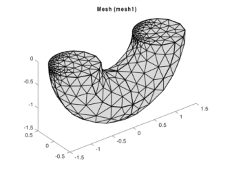
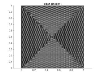
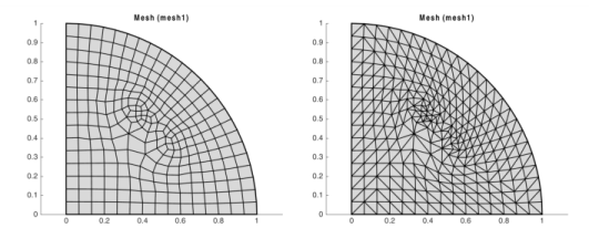
Given a mesh consisting only of simplex elements (lines, triangles, and tetrahedra) you can create a finer mesh using the feature Refine. Enter this command to refine the mesh:

By specifying the property tri, either as a row vector of element numbers or a 2-row matrix, the elements to be refined can be controlled. In the latter case, the second row of the matrix specifies the number of refinements for the corresponding element.

The refinement method is controlled by the property rmethod. In 2D, its default value is regular, corresponding to regular refinement, in which each specified triangular element is divided into four triangles of the same shape. Setting rmethod to longest gives longest edge refinement, where the longest edge of a triangle is bisected. Some triangles outside the specified set might also be refined in order to preserve the triangulation and its quality.

In 3D, the default refinement method is longest, while regular refinement is only implemented for uniform refinements. In 1D, the function always uses regular refinement, where each element is divided into two elements of the same shape.

	For stationary or eigenvalue PDE problems you can use adaptive mesh refinement at the solver stage with the adaption solver step. See Adaption in the COMSOL Multiphysics Programming Reference Manual.

Use the CopyEdge feature in 2D and the CopyFace feature in 3D to copy a mesh between boundaries.

	It is only possible to copy meshes between boundaries that have the same shape. However, a scaling factor between the boundaries is allowed.

The following example demonstrates how to copy a mesh between two boundaries in 3D and then create a swept mesh on the domain:

The algorithm automatically determines how to orient the source mesh on the target boundary. The result is shown in Figure 3-13.

To explicitly control the orientation of the copied mesh, use the EdgeMap attribute. The command sequence:

copies the mesh between the same boundaries as in the previous example, but now the orientation of the source mesh on the target boundary is different. The domain is then meshed by the free mesh, resulting in the mesh in Figure 3-14. In this case it is not possible to create a swept mesh on the domain because the boundary meshes do not match in the sweeping direction.

Use the Convert feature to convert meshes containing quadrilateral, hexahedral, or prism elements into triangular meshes and tetrahedral meshes. In 2D, the function splits each quadrilateral element into either two or four triangles. In 3D, it converts each prism into three tetrahedral elements and each hexahedral element into five, six, or 28 tetrahedral elements. To control the method used to convert the elements, use the property splitmethod.