Working with Geometry Sequences

This section shows how to create geometry sequences using the syntax outlined in The Geometry Sequence Syntax. This section has these examples:

	For more information about geometry modeling, see the Geometry chapter in the COMSOL Multiphysics Reference Manual.

From the MATLAB command prompt, create a 1D geometry model by adding a geometry sequence and then adding geometry features. The last step is to run the sequence using the run method.

First create a model object:

Then continue with the commands:

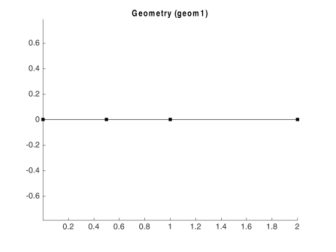
This creates a geometry sequence with a 1D solid object consisting of vertices at x = 0, 1, and 2, and edges joining the vertices adjacent in the coordinate list.

Then enter:

to add a point object located at x = 0.5 to the geometry.

To plot the result, enter:

Use a model object with a 2D geometry. Enter:

Continue by creating a rectangle with side length of 2 and centered at the origin:

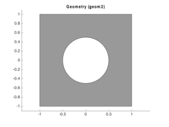
The property size describes the side lengths of the rectangle and the property pos describes the positioning. The default is to position the rectangle about its lower-left corner. Use the property base to control the positioning.

Create a circular hole with a radius of 0.5 centered at (0, 0):

The property r describes the radius of the circle, and the property pos describes the positioning.

	The property pos could have been excluded because the default position is the origin. The default is to position the circle about its center.

Drill a hole in the rectangle by subtracting the circle from it:

A selection object is used to refer to the input object. The operators +, *, and - correspond to the set operations union, intersection, and difference, respectively.

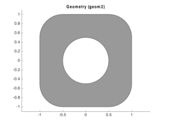
The Compose operation allows you to work with a formula. Alternatively use the Difference operation instead of Compose. The following sequence of commands starts with disabling the Compose operation:

Run the geometry sequence to create the geometry and plot the result:

Continue with rounding the corners of the rectangle with the Fillet operation:

Run the sequence again:

The geometry sequence is updated with rounded corners. To view the result, enter:

Use the following commands to create six open curve segments that together form a closed curve:

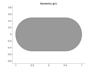
The objects c1, c2, c3, c4, c5, and c6 are all curve2 objects. The vector [1 w 1] specifies the weights for a rational Bézier curve that is equivalent to a quarter-circle arc. The weights can be adjusted to create elliptical or circular arcs.

Convert the curve segments to a solid with the following conversion command:

Then issue a final run command:

This section shows how to create 3D solids using work planes and Boolean operations.

Create a 3D geometry with an xy work plane at z = 0:

Add a rectangle to the work plane, then add fillet to its corners:

Add another yz work plane, at x = 0.5:

Revolve the triangle from the yz work plane:

Add the difference operation that computes the final 3D geometry:

To run the sequence, enter:

To view the geometry enter: