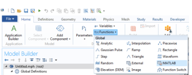
Defining a MATLAB® Function in the COMSOL® Model

To evaluate a MATLAB function from in the COMSOL Multiphysics model you need to add a MATLAB node in the model object where the function name, the list of the arguments, and, if required, the function derivatives, are defined.

To add a MATLAB function node, on the toolbar, click and select (

The window of the node has these sections:

•

, where you declare the name of the MATLAB functions and their arguments.

•

, where you define the derivative of the MATLAB functions with respect to all function arguments.

•

, where you can define the limit of the arguments value in order to display the function in the COMSOL Desktop Graphics window.

This figure illustrates the window for :

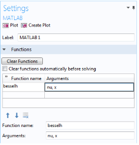
Under , you define the function name and the list of the function arguments.

In the table columns and rows, enter the and the associated function . The table supports multiple function definitions. You can define several functions in the same table or add several nodes, as you prefer.

Any function that you want to call using a node must fulfill the following requirements:

For example, functions such as + and - (plus and minus) work well on vector inputs, but matrix multiplication (*, mtimes) and matrix power (^, mpower) do not. Instead, use the elementwise array operators .* and .^. See also Function Input/Output Considerations.

It is good practice to test your own functions and any MALTLAB functions that you want to call from COMSOL Multiphysics by running them on the MATLAB command line using vectors with suitable values as inputs. For example, using besselj, a Bessel function of the first kind:

Here there are no errors, and the size of the input and output is the same.

As another example, test the corrcoef function for computing correlation coefficients:

There are no errors when calling corrcoef using vector inputs, but the result does not have the same size as the input and hence a call to corrcoef in this way will not work.

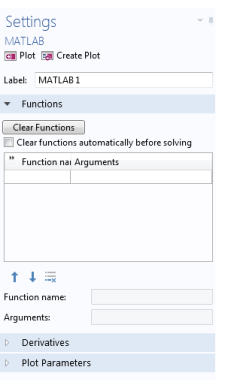
Click the button (

) to display a plot of the function.

Click the button (

) to create a plot group under the node.

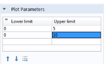
To plot the function you first need to define limits for the arguments. Expand the section and enter the desired value in the and columns. In the table the number of rows correspond to the number of input arguments of the function. The first input argument corresponds to the top row.

In case there are several functions declared in the table, only the function that has the same number of input arguments as the number of filled in rows in the table is plotted.

If several functions have the same number of input arguments, the first function in the table (from top to bottom) is plotted. Use the (

) and (

) buttons to change the order of functions in the table.

Assume that you want to use MATLAB’s Bessel function of the third kind (Hankel function) in a COMSOL model. Add a MATLAB function node, then define the following settings:

Function Name	Arguments
besselh	nu, x

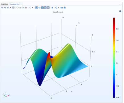
To plot the function you need first to define the lower and upper limits for both nu and x. In the table set the first row (which corresponds to the first argument nu) of the column to 0 and the column to 5 and set the second row (corresponding of x) of the column to 0 and the column to 10: