Apparent Heat Capacity Method
The apparent heat capacity formulation provides an implicit capturing of the phase change interface, by solving for both phases a single heat transfer equation with effective material properties. The latent heat of phase change is taken into account by modifying the heat capacity.
It applies well to materials showing a mushy zone around the phase change interface. And it allows topology changes of the phase change interface.
The Phase Change Material domain condition should be used on both phases domains, to solve the heat equation after specifying the properties of the phase change material according to the apparent heat capacity formulation.
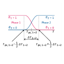
Instead of adding a latent heat L in the energy balance equation exactly when the material reaches its phase change temperature Tpc, it is assumed that the transformation occurs in a temperature interval between Tpc − ΔT ⁄ 2 and Tpc + ΔT ⁄ 2. In this interval, the material phase is modeled by a smoothed function, θ, representing the fraction of phase before transition, which is equal to 1 before Tpc − ΔT ⁄ 2 and to 0 after Tpc + ΔT ⁄ 2. The density, ρ, and the specific enthalpy, H, are expressed by:
where the indices 1 and 2 indicate a material in phase 1 or in phase 2, respectively. Differentiating with respect to temperature, this equality provides the following formula for the specific heat capacity:
which becomes, after some formal transformations:
Here, θ1 and θ2 are equal to θ and 1−θ, respectively. See Figure 4-2 for details.
Figure 4-2: Phase indicators, phase change temperature, and transition interval.
The mass fraction, αm, is defined from ρ1, ρ2 and θ according to:
It is equal to 1 ⁄ 2 before transformation and 1 ⁄ 2 after transformation. The specific heat capacity is the sum of an equivalent heat capacity Ceq:
and the distribution of latent heat CL:
In the ideal case, when 1 − θ is the Heaviside function (equal to 0 before Tpc and to 1 after Tpc), dαm ⁄ dT is the Dirac pulse.
Therefore, CL is the enthalpy jump, L, at temperature Tpc that is added when you have a pure substance.
The latent heat distribution CL is approximated by
so that the total heat per unit volume released during the phase transformation coincides with the latent heat:
The latent heat, L, can depend on the absolute pressure but should not depend on the temperature.
Finally, the apparent heat capacity, Cp, used in the heat equation, is given by:
and the ratio of specific heats, γ, is:
The effective thermal conductivity reduces to:
and the effective density is:
To satisfy energy and mass conservation in phase change models, particular attention should be paid to the density in time simulations. When the fluid density is not constant over time, for example, dependent on the temperature, the transport velocity field and the density must be defined so that mass is conserved locally.
The Moving Mesh Interface (described in the COMSOL Multiphysics Reference Manual) can be used to account for model deformation.
Phase Change in Solid Materials
When phase change is considered in solid materials, the density is defined on the material frame. Therefore a single density should be defined for the different phases to ensure mass conservation on the material frame:
The expression of the specific enthalpy, H, simplifies to:
The apparent heat capacity, Cp, used in the heat equation, is given by:
where the mass fraction is: