In the Vibration Fatigue evaluation, only deterministic vibration can be simulated; random vibration analysis is outside its scope.

When computing a stress state history at forced vibration, two cases have to be considered. The first one represents operating conditions when a component is only subjected to an excitation frequency. The second case represents conditions when a component subjected to an excitation frequency and additional static loads, such as gravity or prestress. The excitation frequency will force the component to vibrate back and forth thus causing an alternating stress that can be seen as an amplitude stress state, Σa. The stress response from the stationary loads causes a constant stress state in the component, that can be seen as a mean stress state, Σm. The stress response from both load mechanisms gives a full stress tensor denoted Σ.

Since the S-N curve is heavily influenced by the R-value, R, which in turn depends on the mean stress and the stress amplitude, the stress state from both load mechanisms must be considered.

When no static loads are present, the stress state at each excitation frequency can be computed using a single Frequency Domain study. For each excitation frequency the stress state is

where p is the number of excitation frequency, while the argument t is the time. The time dependence is in this case harmonic.

In the presence of static loads, for example self-weight, a Prestressed Analysis, Frequency Domain study computes both the mean stress state, Σm, and the amplitude stress state, Σa, for each excitation frequency. The stress state at a given excitation frequency is given by

The first step in a fatigue evaluation is the transformation of the stress state at a certain excitation frequency into a fatigue controlling stress, σ, which is a scalar used to evaluate fatigue life from the S-N curve.

The mean stress is computed from the stress state caused by the static loads. Since these loads are constant at all excitation frequencies, the resulting stress state, Σm, is also constant and so is the mean stress, σm. When the option Directional stress is used, the mean value is taken as the normal stress on the plane defined by the Direction vector. For example, if the stress in the x direction is examined then σm = σxx.

In case of Signed von Mises, the mean stress is computed using the von Mises equivalent stress from the static load case.

where i is the imaginary unit. The modulus of a complex stress, rkl, is the amplitude stress for the stress tensor component, while the argument of the complex number, θkl, is the phase shift of a stress component. These variables are computed using

Thus, the stress component varies between rkl and -rkl during one cycle and the stress history is defined by

where ω is the angular frequency that is related to the excitation frequency through ω = 2πf.

The Directional stress option considers a stress normal to a given plane. If, for example, the yz-plane is considered, the normal stress is given by

and the fatigue stress amplitude is taken as the highest stress during the excitation period which is the modulus of σxx. Thus,

The Signed von Mises option computes an equivalent stress which depends on all components of the complex stress tensor. The square of the von Mises stress is given by

Both the squares of the individual stress components, Equation 3-7, and the cross products between the two normal stress components, Equation 3-8, can be written on the general form

where for i = k and j = l or for i = j and k = l

The square of the equivalent stress, Equation 3-6, can be rewritten into following form

The S-N curve provides the stress amplitude as a function of the R-value and the number of cycles to failure, N. Since both the fatigue mean stress and the fatigue stress amplitude are known for each excitation frequency, the R-value is computed by

where the subscript p denotes the frequency dependence. Once the stress amplitude and R-value are known for each excitation frequency, fp, the limiting number of cycles at each excitation frequency, Np, is extracted from the S-N curve. The relation between the duration time of the excitation at a given frequency, tp, and the number of cycles experienced is given by

The partial damage from a given excitation frequency is simply the ratio ni/Ni. Following the Palmgren-Miner linear damage rule the damage from all excitation frequencies is summarized using

where q denotes the number of excitation frequencies. The fatigue usage factor fus denotes the cumulative damage. Values below 1 means that fatigue is not expected during the analyzed frequency sweep.

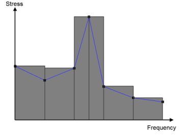
The number of frequency blocks depends on the number of frequencies, F, specified in the Frequency Domain study, where the stress response is computed at each frequency. A frequency block stretches between two evaluation frequencies and the stress response at the evaluation frequency that gives a higher stress value is used in the computation of the damage. As an example, in the figure below the stress response is computed at 7 frequencies in the Frequency Domain study. This gives 6 evaluation blocks. Note that blocks do not need to stretch over equal frequency intervals. If a computation is made around an eigenfrequency the stress response at this evaluation frequency will be used in fatigue computation for the both neighboring blocks of the evaluation frequency. The use of the higher stress for the entire block gives a conservative estimate. Due to the nonlinear dependence between stress and fatigue life, the larger stress cycles will dominate the fatigue life prediction.

where tb is the time duration of a block, fp+1 is the higher evaluation frequency, and fp is the lower evaluation frequency. The number of cycles in each block, nb, is evaluated using

Note that the subscript b is the block number while p is the frequency excitation number. The relation between these two is b = p − 1.

In an experimental frequency sweep over a large range of frequencies, it is common that the rate of frequency change is given in octaves, which is a doubling of the frequency. The reason behind this choice is to give the same time for doubling of frequencies when evaluating frequencies of different magnitudes. The rate of change is then a logarithmic sweep rate, Cl, that is a proportionality constant between the binary logarithm of the excitation frequency and the time. The binary logarithm is the logarithm to the base 2. The relation between the time it takes to sweep between two frequencies, which in the computation is the block time, is given by