The Fatigue Module has the Morrow Model and Darveaux Model to predict fatigue based on the Energy Dissipation.

Morrow (Ref. 6) proposed an exponential fatigue relation in elastoplastic materials given by

where ΔWd is the range of the dissipated energy density during one cycle, Nf is the number of load cycles until failure (one fatigue cycle consists of two reversals), and Wf' and m are material constants.

In the original work, ΔWd was taken as the range of the plastic dissipated density. This has been extended in the Fatigue Module where the Morrow model can be used with other dissipated energies, depending on the parameter Energy type selected under Fatigue Model Selection for the Energy-Based node. The dissipated energy is evaluated according to Table 3-5 where ΔWc is the range of the creep dissipated energy density during one cycle and ΔWp is the range of the plastic dissipated energy density during one cycle.

Darveaux (Ref. 7) relates fatigue life to a volume average of dissipated energy according to

where the first term in the equation represents the number of cycles necessary to initiate fatigue and the second term defines the number of cycles during crack growth. N is the number of cycles necessary to grow a crack until it has reached the size a. K1, k2, K3, and k4 are material constants. The average dissipated energy density range ΔWave is based on the dissipated energy density range ΔWd that is evaluated over the material volume V. The integration of the energy density reduces the sensitivity to meshing since singularities can be expected at sharp geometrical changes, corners, or domain interfaces. Phenomenologically this is explained by the fact that a crack propagates through a layer and the energy dissipated in that layer controls fatigue.

The dissipated energy density range can take different values specified by the Energy type parameter as defined for the Energy-Based node. Available options are summarized in Table 3-5.

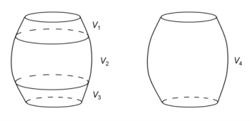
The computation of ΔWave is determined by the parameter Volume integration. When Individual domains is selected, the average value is calculated over each geometrical domain specified in the selection. When Entire selection is selected, a single average value is calculated based on the dissipated energies in all domains in the selection. The difference between these two options is illustrated in Figure 3-14, where two equal solder joints are shown. One of them is subdivided into three geometrical domains with volumes V1, V2, and V3 while the second one consists of only one domain with volume V4. Since both joints have the same dimensions, .

Assume that both solder joints are subjected to the same load and boundary conditions. Then the same energy is dissipated in them. When the model with three geometrical domains is evaluated, the option Individual domains calculates

while the option Entire selection calculates

For selections that consist of one geometrical domain both the options of the Volume average method parameter calculate the same result.