Layered Material
In the Layered Material node (), you can specify the properties of a multilayer laminate. It is used when defining the properties of the following features:
Layered Linear Elastic Material in the Shell interface (requires the Composite Materials Module).
Thin Layer in the Heat Transfer in Solids interface.
A Layered Material node can be present in two locations in the Model Builder:
The most common place is under Global Definitions>Materials. When you reference a layered material from a physics interface, you do it indirectly through either a Layered Material Link or a Layered Material Link (Subnode) under Materials in the current component.
Layer Definition
In this table you specify the properties of each layer.
Click the Add button () to add another table row. Use the Move up (), Move down (), and Delete () buttons to organize the table as needed. To completely reset the table to its default state, you can use the Reset to Default button ().
Conceptually, the layers are ordered from bottom to top of the laminate. Enter the following data in the table:
Layer
Here you can assign a name to the layer for future reference. The default is a sequential numbering: Layer 1, Layer 2, and so on.
Material
Select any available material. If the Layered Material node is located under Global Definitions, the list contains only global materials. If the Layered Material node is used as a subnode to a Layered Material Stack, also materials defined under Materials in the component are available.
When you have a certain row in the table selected, you can access three shortcuts:
Click the Blank Material () button to add a new blank material under global materials. The material is referenced in current row of the Material column.
Click the Add Material from Library () button to add a new material under global materials from Material Libraries. The material is referenced in current row of the Material column.
Click the Go to Material () button to jump to the definition of the material selected on the current row.
When you add a new row to the table, the same material as on the previous row is selected. This means that if you have many, not adjacent, layers with the same material, it is more efficient to initially add all layers with that same material. Then you can go back and change the material for some layers. Alternatively, you can reorder the layers using the Move up () and Move down () buttons.
Rotation
If the material in the layer is orthotropic or anisotropic, enter the angle in degrees (positive counterclockwise) from the first principal axis of the laminate to the first principal axis of the layer. Even for an isotropic material, the orientation can matter for result presentation, since it affects the interpretation of for example stress tensor components.
Thickness
Enter the thickness of the layer (default unit: m). The thickness can be numeric value or a scalar parameter.
Mesh Elements
In the physics interfaces, the layered materials are handled through the concept of a virtual extra dimension. For a layered material defined on a boundary, you can think of that as an extra coordinate in the normal direction. Enter the number of elements that you want in the extra dimension for the layer.
Interface Property
In some physics features, not only the layers themselves but also the interfaces between them are important. In such a case, you can assign materials to the interfaces in this table. The number of interfaces is one more than the number of layers because the free top and bottom surfaces of the laminate are also considered as interfaces.
In most cases, you do not need to enter anything in this section.
Interface
This is the interface name, for future reference. As a default, the interface name is constructed from the names of the two adjacent layers. For the top and bottom interfaces, the labels “up” and “down” are used for the two exterior sides.
You can rename the interfaces. This is, however, seldom needed.
Position
This column shows the location of the interface. The distance is counted from the bottom of the laminate. The column is for information only, and cannot be modified.
Material
Select the material of the interface. You only need to assign materials to the interfaces that are explicitly referenced by physics features. The default is to take the material From layer. The interface material properties are then computed from the adjacent layers’ material properties.
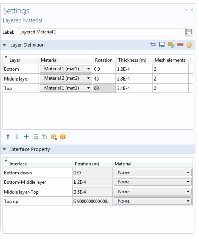
Figure 9-8 shows an example of the settings for a layered material. The layer names have been entered manually, whereas the interfaces have retained their default names.
Figure 9-8: Settings for a material with three layers.
You can save the laminate definition to a text file by clicking the Save Layers to File () button. For the example above, the text file has the following contents:
Bottom mat1 0.0 1.2E-4 2
"Middle layer" mat2 45 2.3E-4 2
Top mat1 60 3.4E-4 2
To load a text file on this format, click the Load Layers from File () button. For complex laminates, it may be easier to start by creating the text file representation in a text editor, than to enter the data in the GUI.
When loading a file, the second column containing the material tag is ignored. The reason is that there is no way to ascertain that a material tag like ‘mat2’ would point to the same material in another context. You can even load a file where that column is absent.
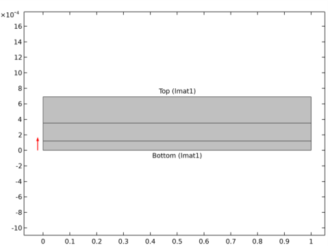
You have two options for visualizing the laminate defined in the Layered Material node. To see the thickness of each layer, click the Layer Cross Section Preview () button. This will give a plot like the one shown in Figure 9-9.
Figure 9-9: The layer cross section plot for a material with three layers.
You can also click the downward pointing arrow to choose Layer Cross Section Preview () or Create Layer Cross Section Preview (), which adds the preview plot as a new plot group under Results. By clicking the Layer Cross Section Preview () button, you get a preview plot of the single layer material, including the location of the reference surface. This plot looks similar to Figure 9-12, but there is only a single layer.
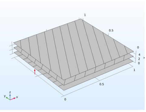
To visualize the layer orientations, click the Layer Stack Preview () button. In Figure 9-10, an example of such a plot is shown. The x-axis corresponds to the principal laminate direction, and the stripes indicate the principal direction of each layer. You can also click the downward pointing arrow to choose Layer Stack Preview () or Create Layer Stack Preview (), which adds the preview plot as a new plot group under Results. Click the Create Layer Stack Plot button () to add the preview of the layer stack as a new plot group under Results.
Figure 9-10: The layer stack preview plot for a material with three layers.
Preview Plot Settings
In this section, you can fine-tune the display in the preview plots.
In the Distance between the orientation lines text field, you can enter a value for the spacing of the stripes showing the orientation of the principal orientation of the layer. The layer itself is always drawn as a square with the unity side length. If you clear the corresponding check box, no orientation lines are drawn.
The value of the Thickness-to-width ratio is used by both types of preview plots.
In a layer stack preview plot, it controls the height of the stack in the z direction. For laminates with many layers, you may need to increase this value.
Clear the Shows labels in cross section plot check box to remove the text labels showing layer names and materials.