Water purification is a multiple step process for turning natural water into drinking water. At least one step must be a disinfectant step. One way to achieve efficient disinfection in an environmentally friendly way is to use ozone. A typical ozone purification reactor is about 40 m long and resembles a maze with partial walls or baffles that divide the space into room-sized compartments (Ref. 1). When water flows through the reactor, turbulent flow is created along its winding path around the baffles toward the exit pipe. The turbulence mixes the water with ozone gas, which enters through diffusers just long enough to deactivate micropollutants. When the water leaves the reactor, the remaining purification steps filter off or otherwise remove the reacted pollutants.

When analyzing an ozone purification reactor, the first step is to get an overview of the turbulent flow field. The results from the turbulent-flow simulation can then be used for further analyses of residence time and chemical species transport and reactions. This step requires adding more physics features to the model. The current application solves for turbulent flow in a water treatment reactor using the Turbulent Flow, k-ε interface.

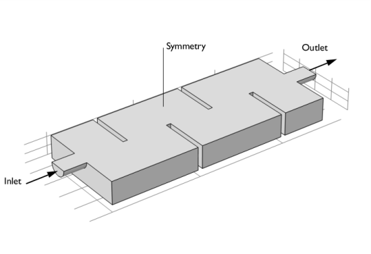
The model geometry along with some boundary conditions is shown in Figure 10. The full reactor has a symmetry plane, which is utilized to reduce the size of the component.

Based on the inflow velocity, which is 0.1 m/s, and a length scale L equal to the diameter of the inlet, the Reynolds number is

Here ν is the kinematic viscosity. The high Reynolds number clearly indicates that the flow is turbulent and a turbulence model must be applied. In this case, you will use the k-ε model. It is commonly used in industrial applications, because it is both relatively robust and computationally inexpensive compared to more advanced turbulence models. One major reason to why the k-ε model is inexpensive is that it employs wall functions to describe the flow close to walls instead of resolving the very steep gradients there. All boundaries are walls in Figure 10 except the inlet, the outlet, and the symmetry plane.

The velocity field in the symmetry plane is shown in Figure 11. The jet from the inlet hits the edge of the first baffle, which splits the jet. One half creates a strong recirculation zone in the first “chamber”. The other half continues downstream into the reactor and gradually spreads out. The velocity magnitude decreases as more fluid is entrained into the jet.

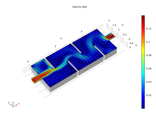
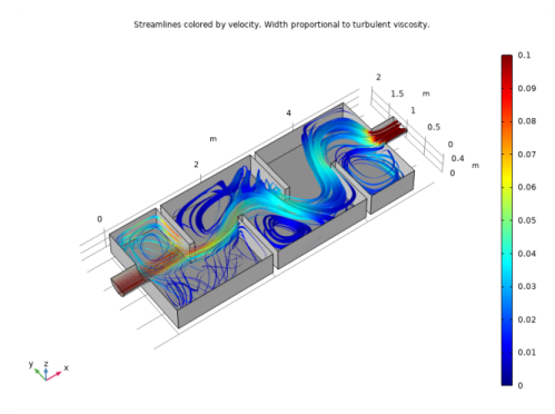
Figure 12 gives a more complete picture of the mixing process in the reactor. The streamlines are colored by the velocity magnitude, and their widths are proportional to the turbulent viscosity. Wide lines hence indicate a high degree of mixing. The turbulence in this model is mainly produced in the shear layers between the central jet and the recirculation zones. The mixing can be seen to be relatively weak near the entrance to the reactor and to increase further downstream.