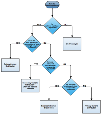
Under the assumption of a linear relation of current density to electric field, Ohm’s law is obeyed for the electrolyte current. This is the assumption of primary current distribution, where one also assumes infinitely fast electrodes kinetics, resulting in negligible potential drops over the electrode-electrolyte interfaces. If the electrode reaction kinetics proceed at a finite rate, then the system has a secondary current distribution. In the cases of more advanced nonlinear charge conservation equations being required and concentration-dependent electrode polarization, the system is described as obeying tertiary current distribution.

In some applications, especially within the field of electroanalysis, the potential gradients in the electrolyte are so small that the spatial distribution of current in the electrolyte is not solved for. Such models are instead centered around the interplay of electrode kinetics and transport (by diffusion) of the reacting species in the vicinity of the electrode.