Tutorial Example: Pesticide Transport and Reaction in Soil
Aldicarb is a commercial pesticide, used on a variety of crops, including cotton, sugar beet, citrus fruits, potatoes, and beans. People may be exposed to aldicarb primarily through the ingestion of contaminated water and food.
This example looks at the degradation kinetics of aldicarb and its toxic by-products, investigating both the degradation time-scale as well as the spatial concentration distribution of toxic components.
In the first model the chemical compounds are contained in a water pond, treated as a perfectly mixed system.
The second model tracks the detailed distribution of chemicals in the soil as the pesticide leaches out of the pond and is transported by water through the surrounding soil.
Investigating a Perfectly Mixed System
First consider the water pond as a perfectly mixed system. Aldicarb degrades by transformation to the corresponding sulfoxide and sulfone (which are both relatively toxic), and it is detoxified to oximes and nitrile by hydrolysis.
The chain of reactions is illustrated in Figure 2.
Figure 2: Reaction pathways of aldicarb degradation. The toxicity is indicated by its LD50 value (mg/kg), signifying the median lethal dose.
Each of the unimolecular reactions outlined in Figure 2 has a rate expression rj of the form
(1)
In this example, the species concentrations cj are given in units of mol/m3, and the rate constants kj are expressed in 1/day.
The reactions for the chemical species are given by:
(2)
(3)
(4)
(5)
(6)
(7)
Solving this set of coupled ODEs provides information on the time scales of the degradation processes in a closed and perfectly mixed system.
Results
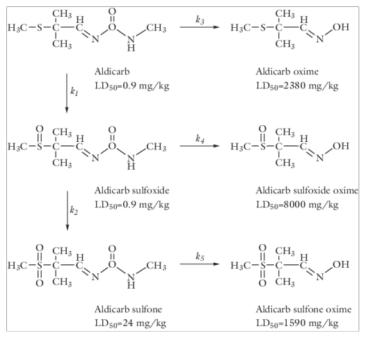
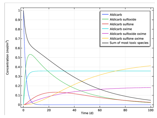
The results of the perfectly mixed system, shown in Figure 3, portrait the concentration profiles of aldicarb and its decay by-products and the concentration transients of the three most toxic species — aldicarb, aldicarb sulfoxide, and aldicarb sulfone — as well as their sum (see Figure 2 for LD50 values). Only small amounts of aldicarb remain in the pond after 10 days. Considering the summed-up contributions, contamination levels in the water pond remain high even after several months.
Figure 3: Concentration profiles as reactions occur during a 100 day time period. Concentration transients of the most toxic species, aldicarb (ca), aldicarb sulfoxide (casx), aldicarb sulfone (casn), and the sum of them
Investigating a 2D Model
The results shown in Figure 3 indicate that the concentration of aldicarb, in a pond treated as a perfectly mixed system, decay to less than 1% the initial concentration after 10 days. Consider this time scale as a reference for a more detailed model.
The spatial-dependent model focuses on the concentration of the highly toxic species aldicarb (ca), aldicarb sulfoxide (casx), and aldicarb sulfone (casn). Therefore, you can disregard the mass balances for the hydrogenolysis products (cao, csxo, and csno).
In this more detailed model, you assume that aldicarb moves from the pond into a relatively dry soil. In the soil, the aldicarb decomposes into aldicarb sulfoxide and aldicarb sulfone according to the mechanism illustrated in Figure 2. In addition, the pesticide and its decay by-products are transported by convection, dispersion, adsorption, and volatilization.
Model Geometry
In this application, water is ponded by a ring sitting on the ground. The soil is represented by two layers. The top layer is slightly less permeable than the bottom one, which sits on an almost impervious rock bed. The water moves through the bottom of the ring into the soil. The water level in the ring is known, as is the initial distribution of pressure heads in the soil. There is no flow through the vertical walls or the air-soil surface.
Aldicarb moves with the water from the pond into the soil at a constant concentration. Once in the soil, the chemicals react and adsorb onto soil particles. Aldicarb and the aldicarb sulfone volatilize to the atmosphere. The adsorption, biodegradation, and volatilization proceed is proportional to the aqueous concentrations.
The soil is initially pristine with zero concentration of the involved chemicals. At the ground surface outside the ring, aldicarb and aldicarb sulfone volatilize to the atmosphere.
The left vertical axis is a line of symmetry. The other boundaries are posed such that the solutes can freely leave the soil column with the fluid flow. Model the problem with 2D axisymmetry and track the solute transport for 10 days.
Figure 4: Geometry of the infiltration ring and soil column.
Fluid Flow
Richards’ equation governs the saturated-unsaturated flow of water in the soil. The soil pores are connected to the atmosphere, so you can assume that pressure changes in the air do not affect the flow and thus use Richards’ equation. Given by Ref. 1, Richards’ equation given in pressure head reads
(8)
where C denotes specific moisture capacity (m-1); Se is the effective saturation of the soil (dimensionless); S is a storage coefficient (m-1); Hp is the pressure head (m), which is proportional to the dependent variable, p (Pa); t is time; K equals the hydraulic conductivity (m/s); D is the direction (typically, the z direction) that represents the vertical elevation (m).
To be able to combine boundary conditions and sources with the Darcy’s Law and Fracture Flow interfaces, COMSOL Multiphysics converts Richards’ equation to SI units and solves for the pressure variable (SI unit: Pa).
Hydraulic head, H, pressure head, Hp, and elevation D are related to pressure p as
(9)
Also, the soil permeability κ (SI unit: m-2) and hydraulic conductivity K (SI unit: m/s) are related to the fluid viscosity μ (SI unit: Pa·s) and density ρ (SI unit: kg/m3), and to the acceleration of gravity g (SI unit: m/s2) by
(10)
In this model, the specific moisture capacity Cm and the effective saturation Se are taken from the van Genuchten retention model (Ref. 2). For more details see The Richards’ Equation interface in the Subsurface Flow Module User’s Guide.
Mass Transport
The governing equation for solute transport describes advection and dispersion of a sorbing, volatilizing, and decaying solute in variably saturated soil.
(11)
The Transport of Diluted Species in Porous Media interface implements the equation above for one or several species. It describes the time rate of change in two terms: c denotes dissolved concentration (mol/m3) and cP the mass of adsorbed contaminant per dry unit weight of soil (mg/kg). Further, θ denotes the volume fraction of fluid (dimensionless), and ρb is the soil’s bulk density (kg/m3). Because ρb amounts to the dried solid mass per bulk volume, the term ρbcP gives the solute mass attached to the soil as the concentration changes with time.
Solute spreading also includes mechanical dispersion in water plus molecular diffusion for water and air. These three processes appear in the liquid-gas dispersion tensor, whose entries are
(12)
(13)
In these equations, DLGii are the principal components of the water-air dispersion tensor; DLGij and DLGji are the cross terms; α is the dispersivity (m) where the subscripts “1” and “2” denote longitudinal and transverse dispersivity; Dm and DG (m2/d) are molecular diffusion coefficients; and τL and τG give the tortuosity factors for water and air, respectively.
The three solutes — aldicarb, aldicarb sulfoxide, and aldicarb sulfone — have different decay rates, RLi, partition coefficients, kPi, and volatilization constants, kGi. All the three solutes attach to soil particles, but only aldicarb and aldicarb sulfone volatilize; aldicarb sulfoxide does not.
Results
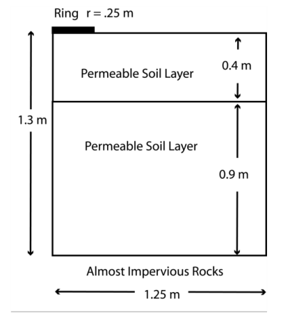
The following results come from the space- and time-dependent model. Figure 5 shows the fluid flow in soil after 0.3 days (left) and 1 day (right). The plots illustrate the wetting of the soil with time. As indicated by the arrows, the fluid velocities are relatively high beneath the ponded water.
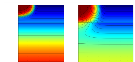
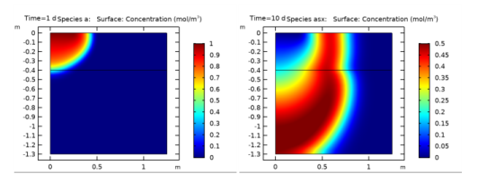
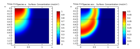
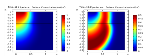
Figure 5: The effective saturation (surface plot), pressure head (contours), and flow velocity (arrows) in a variably saturated soil after 0.3 days (left) and 1 day (right).
Figure 6 through Figure 8 show the concentration distributions of aldicarb and the equally toxic aldicarb sulfoxide after 1, 5, and 10 days of infiltration. Consistent with the evolving flow field, the main direction of transport is in the vertical direction.
Figure 6: Concentration of aldicarb (left) and aldicarb sulfoxide (right) after 1 day.
Figure 7: Concentration of aldicarb (left) and aldicarb sulfoxide (right) after 5 days.
Figure 8: Concentration of aldicarb (left) and aldicarb sulfoxide (right) after 10 days.
The distribution of aldicarb has clearly reached steady-state conditions after 10 days, a time frame that was also predicted by the ideal reactor model (see Figure 2). Results also show that the soil contamination is rather local with respect to the aldicarb source. The aldicarb sulfoxide, on the other hand, can be expected to affect a considerably larger soil volume for a significantly longer time.
References
1. J. Bear, Hydraulics of Groundwater, McGraw-Hill Inc., 1978.
2. M.Th. van Genuchten, “A closed-form equation for predicting the hydraulic of conductivity of unsaturated soils”, Soil Sci. Soc. Am. J., vol. 44, pp. 892–898, 1980.