In COMSOL Multiphysics you can model contact between a group of boundaries in 2D or 3D. There are two algorithms available: an augmented Lagrangian method and a penalty method.

In the augmented Lagrangian method, the system of equations is solved in a segregated way. Augmentation components are introduced for the contact pressure Tn and the components Tti of the friction traction vector Tt. An additional iteration level is added where the usual displacement variables are solved separated from the contact pressure and traction variables. The algorithm repeats this procedure until it fulfills a convergence criterion.

In the following equations F is the deformation gradient matrix. When looking at expressions evaluated on the destination boundaries, the expression map (E) denotes the value of the expression E evaluated at a corresponding source point, and g is the current gap distance between the destination and source boundary.

Both the contact map operator map (E) and the gap distance variable are defined by the contact element elcontact. For each destination point where the operator or gap is evaluated, a corresponding source point is sought by searching in the direction normal to the destination boundary.

It is possible to add an offset value both to the source (osrc), and to the destination (odst). If an offset is used, the gap will be computed with the geometry treated as larger (or smaller, in the case of a negative offset) than what is actually modeled. The offset is given in a direction normal to the boundary. It can vary along the geometry, and may also vary in time (or by parameter value when using the continuation solver).

The effective gap distance dg used in the analysis is thus

In some cases, the discretization caused by the meshing of curved boundaries will give small irregularities in the gap values. You can then choose to adjust the effective gap by removing the gap values computed in the initial configuration, ginit, smaller than the tolerance Δgap. In this case, the effective gap distance is

When including friction in the contact problem, it is important to keep track of not only the gap in the normal direction, but also the slip between the boundaries in the tangential direction. The slip s since the last converged step is defined as

and Xm,old is the value of Xm in the last converged time or parameter step. The coordinates are material (undeformed) coordinates. The slip vector is thus approximated using a backward Euler step. The deformation gradient F contains information about the local rotation and stretching.

Using the special gap distance variable (solid.gap), the penalized contact pressure Tnp is defined on the destination boundary as

where pn is the user defined normal penalty factor.

The penalized friction traction Ttp is defined on the destination boundary as:

where Tt,trial is defined as

In Equation 3-116, pt is the user defined friction traction penalty factor. The critical sliding resistance, Tt,crit, is defined as

In Equation 3-117, μ is the friction coefficient, Tcohe is the user defined cohesion sliding resistance, and Tt,max is the user defined maximum friction traction.

In the following equation δ is the variation (represented by the test() operator in COMSOL Multiphysics). The contact interaction gives the following contribution to the virtual work on the destination boundary:

where i is the augmented solver iteration number and γfric is a Boolean variable stating if the parts are in contact or not.

where dg is the effective gap distance, pn is the penalty factor, and p0 is the pressure at zero gap. The latter parameter can be used to reduce the overclosure between the contacting boundaries if an estimate to the contact pressure is known. In the default case, when p0 = 0, there must always be some overclosure (a negative gap) in order for a contact pressure to develop.

In case of friction, the tangential force Tt is computed as

This can be viewed as a tangential spring giving a force proportional to the sliding distance. The penalty factor pt can be identified as the spring constant. The sticking condition is thus replaced by a stiff spring, so that there is a small relative movement even if the force required for sliding is not exceeded. The definition of Tt,crit is

The friction coefficient μ is defined as

where μstat is the static friction coefficient, μdyn is the dynamic friction coefficient, vs is the slip velocity, and αdcf is a decay coefficient.

You can model a situation where two boundaries stick together once they get into contact by adding an Adhesion subnode to Contact. Adhesion can only be modeled when the penalty contact method is used. The adhesion formulation can be viewed as if a thin elastic layer is placed between the source and destination boundaries when adhesion is activated.

Using the effective gap distance dg and the slip s, the adhesion formulation defines a displacement jump vector u in the local boundary system as

where Tb-T contains the transform from the global system to the boundary system. In the above expression, the Macaulay brackets indicate the positive parts operator such that

Using the displacement jump vector, the adhesive stress vector f is defined as

where k is the adhesive stiffness. For negative values of dg, the normal component of f is zero, and the contact constraint is resolved by the penalty contact formulation. Notice that a different sign convention is used for the normal stress in the adhesion and contact contributions, where Tn is positive in compression.

The adhesive stiffness k can be defined using three different options: From contact penalty factor, User defined, and Use material data. For the first option, the normal stiffness is set equal to the contact pressure penalty factor pn. The two tangential stiffness components are then assumed to be related to the normal stiffness, so that the stiffness vector equals

where nτ is a coefficient with the default value 0.17. This coefficient can either be input explicitly, or be computed from a Poisson’s ratio. A plane strain assumption is used for this conversion, giving

For the Use material data option, k is calculated from the elastic constants of a fictive layer with a thickness equal to ds.

When adhesion is active, it is possible to break the bond between the source and destination boundaries by adding a Decohesion subnode to Contact. Decohesion modifies the stress vector f defined by Adhesion, but does not explicitly add any new contribution to the to the virtual work on the destination boundary. It thus requires an active Adhesion node.

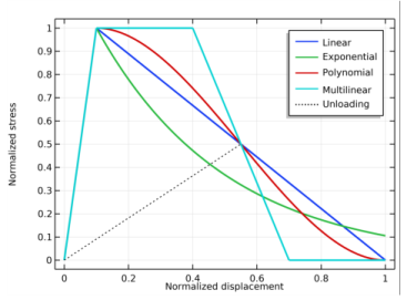
where d is the damage variable. During crack opening (or shearing), the damage variable grows, resulting in a softening behavior of the interface until it eventually breaks when d = 1, see Figure 3-24. If the interface is unloaded, the material follows the linear secant stiffness as defined by the current state of damage. No permanent deformations remain at complete unloading.

The Decohesion subnode implements the second term on the right hand side of Equation 3-118, while the first term is implemented in Adhesion. Notice that in the normal direction, damage only applies to separation of the boundaries, hence the normal contact is unaffected by decohesion.

In the displacement based damage models, the damage variable d is defined using a damage evolution function written in terms of a displacement quantity. Since, in general, the fracture is a combination of mode I and mode II fracture, the model introduces a mixed mode displacement um as the norm of the displacement jump vector.

To keep track of the current state of damage, the maximum value of um over the loading history is defined as

where is and internal degree of freedom that takes the value of um,max at the previous converged solution. The damage variable is then defined as a function of um,max of the form

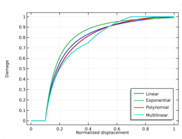
where F-1 is called the damage evolution function and u0m defines the onset of damage. Conceptually, the damage evolution function is the inverse of the softening branch of the traction separation law F. Four different definitions of F-1 are available in the Traction separation law drop-down menu. These damage evolution functions are summarized in Figure 3-23, and the resulting traction separations laws in Figure 3-24.

The Linear option specifies a damage evolution function that gives a bilinear traction separation law as seen in Figure 3-24. It is defined as

where u0m and ufm define the mixed mode initiation of damage and point of complete fracture, respectively. For the initiation of damage, a linear mixed mode criterion gives

where uI and uII are the mode I and mode II displacements, respectively. These are obtained from the displacement jump vector u. The constants u0t and u0s are calculated as

where σt is the tensile strength and σs is the shear strength of the adhesive layer. The normal stiffness kn and the equivalent tangential stiffness kt are obtained from the adhesive stiffness vector k. The mixed mode failure displacement ufm depends on the selected Mixed mode criterion. The Power Law criterion is defined as

and the Benzeggagh-Kenane criterion is defined as

where Gct and Gcs are the tensile and shear energy release rates, respectively. The exponent α is called the mode mixity exponent. From these relations, the mixed mode failure displacement can be calculated. For the power law criterion, the expression is

The Exponential option specifies a damage evolution function that gives a traction separation law which is linear up to the interface strength, and thereafter softens with an exponential curve that reaches zero asymptotically as seen in Figure 3-24.

The mixed mode damage initiation displacement u0m is defined by Equation 3-119 and Equation 3-120. The mixed mode failure displacement ufm is for the power law again given by

The Polynomial option specifies a damage evolution function that gives a traction separation law that is linear up to the interface strength. and thereafter softens with a cubic polynomial curve as seen in Figure 3-24.

The mixed mode damage initiation displacement u0m is defined by Equation 3-119 and Equation 3-120, and the mixed mode failure displacement ufm by Equation 3-121 or Equation 3-122.

The Multilinear option specifies a damage evolution function that gives a traction separation law that is linear up to the interface strength. Thereafter a region of constant stress is introduced before the interface softens linearly as seen in Figure 3-24.

The mixed mode damage initiation displacement u0m is defined by Equation 3-119 and Equation 3-120. The new constant upm defines the end of the region of constant stress and requires the introduction o the shape factor λ. The shape factor defines the ratio between the constant stress part of Gct and the total “inelastic” part of Gct:

Note that the shape factor is similarly defined for shear, and is assumed to be equal for both components. Setting λ = 0 corresponds to the linear separation law. Using the above expression, the stress plateau displacement upi for the respective component can be expressed as

and the failure displacement ufi as

where index i indicates either tension or shear. For the multilinear option, the mixed mode criterion is always linear (α = 1). Hence the mixed mode stress plateau displacement and failure displacements are given as

The energy based damage models provide an alternative formulation that relates the growth of damage to the dissipated mechanical energy of the interface. The formulation is based on the work presented in Ref. 4 and Ref. 5. The derivation starts from a stored energy function

From ψ(u, d), the stress vector f and damage energy release rate Ydm are obtained as

To keep track of the current state of damage, the maximum value of Yd over the loading history is defined as

where is and internal degree of freedom that takes the value of Ydm,max at the previous converged solution. The energy dissipated during the decohesion process is

where Gcm is the critical energy release rate in the sense of fracture mechanics. The overall behavior of the cohesive zone model is then summarized by

where Yd0m defines the damage threshold and F is a monotonically increasing function of the damage variable. From the above, an expression for the damage variable is obtained as

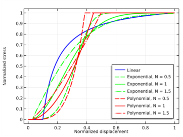
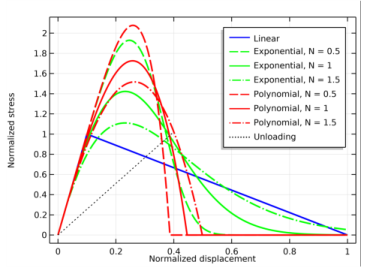
Three different definitions of F-1 are available under the Traction separation law drop-down menu for the energy based damage model. These damage evolution functions are summarized in Figure 3-25, and the resulting traction separations laws in Figure 3-26.

The Linear option specifies a damage evolution function that gives a bilinear traction separation law as seen in Figure 3-26.

For the linear law, the equation constant Ydfm = Gcm. The Exponential option specifies a more general damage evolution function of the following form

where N is a smoothening parameter with a default value equal to 1. The effect of N on the traction separation curve can be seen in Figure 3-26. For the exponential law, Ydfm is defined as

where Γ() is the gamma function. A similar damage evolution function is obtained by the Polynomial option. It gives a generalized version of the traction separation law proposed in Ref. 5 of the form

Left to determine are the two variables Yd0m and Gcm. Their definition require the introduction of a few new concepts related to the mixed mode loading. First, a mixed mode ratio is introduced

where uI and uII are the mode I and mode II displacements, respectively. These are obtained from the displacement jump vector u. The energy release rate of the respective modes are then given by

where G0t and G0s define the damage threshold in tension and shear, respectively. The corresponding criterion for the fracture toughness is

where Gct and Gcs are the critical energy release rates for tension and shear, respectively. The variables α0 and αc are called mode mixity exponents. Using these mode mixture rules results in

Due to the release of energy during decohesion and the softening behavior of the damage models, models may suffer from unwanted mesh dependency. The CZM can suffer from instability leading to non-converging solutions, or bifurcation causing different solutions for different meshes. Such deficiencies may be alleviated by introducing some additional form of regularization. Under the Regularization drop-down menu, it is possible to add the Delayed damage regularization. This option adds a viscous delay to the damage growth, and is available with time dependent studies. The formulation introduces a viscous damage variable dv, and redefines Equation 3-118 so that

where d is the damage variable obtained from any of the available CZM, and τ is the characteristic time that defines the delay of the decohesion. If the viscous damage is used to stabilize a rate-independent decohesion problem, the value of τ must be chosen with care. As a rule of thumb, τ should at least be one or two orders of magnitude smaller than the expected time step. Too large values of τ can introduce significant amounts of extra fracture energy to the model, and the actual energy dissipated due to damage can exceed the defined critical energy release rates by orders of magnitude.

The current value of the viscous damage variable is obtained from numerical integration of Equation 3-123, such that

where Δt is the current time step taken by the time-dependent solver. The value of the viscous damage at the previously converged step is stored as an internal degree of freedom.

where the required values at the previously converged step n are stored as internal degrees of freedom.