Magnetostriction describes the change in dimensions of a material due to a change in its magnetization. This phenomenon is a manifestation of magnetoelastic coupling, which is exhibited by all magnetic materials to some extent. The effects related to magnetoelastic coupling are described by various names. The Joule effect describes the change in length due to a change in the magnetization state of the material. This magnetostrictive effect is used in transducers for applications in sonars, acoustic devices, active vibration control, position control, and fuel injection systems.

The inverse effect accounts for the change in magnetization due to mechanical stress in the material. This effect is also known Villari effect. This effect is mostly useful in sensors.

It is possible to express the relation between the stress S, strain ε, magnetic field H, and magnetic flux density B in either a stress-magnetization form or strain-magnetization form:

where μ0 is the magnetic permeability of free space; cH and sH are the stiffness and compliance matrices measured at constant magnetic field, respectively; and μrS and μrT are the relative magnetic permeabilities measured at constant strain and constant stress, respectively. The matrices dHT and eHS are called piezomagnetic coupling matrices.

You find all the necessary material data inputs within the Magnetostrictive Material node under the Solid Mechanics interface, which are added automatically when you add a predefined Magnetostriction multiphysics interface. Such a node can be also added manually under any Solid Mechanics interface similar to all other material model features. The Magnetostrictive Material uses Voigt notation for the anisotropic material data. More details about the data ordering can be found in the Orthotropic and Anisotropic Materials section.

The following material data corresponds to Terfenol-D at 100 kA/m bias and 30 MPa prestress (Ref. 5):

A commonly accepted micromagnetic description of the magnetostriction is as follows (Ref. 2):

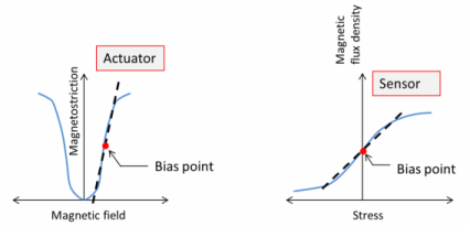
All domains have magnetization of the same magnitude |M| = Ms, but the magnetization can have different orientations characterized by the corresponding direction vector m = M/Ms for each domain. The applied magnetic field changes the domain orientation.

where . Note that the magnetostrictive strain is represented by a deviatoric tensor, that is, tr(εme) = 0. This is because the deformation is related to the magnetic domain rotation, and such process should not change the material volume.

The strain in any direction given by the directional cosines βi can be written as

Using Equation 3-67, one gets

When both magnetization and measurement direction are parallel to the same crystal direction [100], one has m1 = β1 = 1 and all other components are zero, so that

In a similar way for the [111] direction, one has for all components and λ = λ111.

If the strain is measured in [100] direction, while all the magnetization vectors are aligned perpendicular to it, one has only the following two nonzero components: m2 = β1 = 1 and consequently:

For an isotropic material, λ100 = λ111 = λs, and Equation 3-67 becomes

For a polycrystalline material without preferred orientation, the following approximation can be used (Ref. 1):

The strain field is deviatoric, and Equation 3-69 exhibits the same properties as Equation 3-67 at saturation, that is, when |M| → Ms. Equation 3-68 is replaced by

Note that the strain vanishes when |M| → 0, which makes the model applicable in the whole range from full demagnetization to saturation.

For isotropic materials, the magnetostrictive strain is modeled as the following quadratic isotropic form of the magnetization field (Ref. 3):

For isotropic materials, the stiffness matrix cH can be represented in terms of two parameters, for example, using the Young’s modulus and Poisson’s ration. Cubic materials possess only three independent components: c11, c12, and c44.

Using Equation 3-70, one can derive a linear response around a given bias state characterized by a premagnetization vector M0. Thus,

where M1 is a perturbation, and

Nonlinear magnetization in the magnetostrictive material is found from the following nonlinear implicit relation (Ref. 4):

where L is the Langevin function

with χm being the magnetic susceptibility in the initial linear region.

Other possible choices of the L function are a hyperbolic tangent

where H is the applied magnetic field. The second term in Equation 3-72 represents the mechanical stress contribution to the effective magnetic field, and thus to the material magnetization, which is called the Villari effect. The deviatoric stress tensor is related to the strain as

In addition, the magnetization and magnetic field are related to each other and to the magnetic flux density (also called the B-field) by

COMSOL Multiphysics solves for the magnetic vector potential A whose curl yields the vector B-field. The H-field is then obtained as a function of the B-field and magnetization.

The Jiles-Atherton hysteresis model for magnetostrictive materials is available COMSOL Multiphysics. The model assumes that the total magnetization can be represented as a sum of hysteretic and anhysteretic parts, the latter one is given Equation 3-71, thus

Compared to Equation 3-72 and Equation 3-73, the effective magnetic field Heff gets one more term αMan, where α is the interdomain coupling parameter.

where cr is the reversibility parameter, and kp is the pining parameter.

Equation 3-74 can be solved using either a time dependent analysis or a stationary parametric sweep.