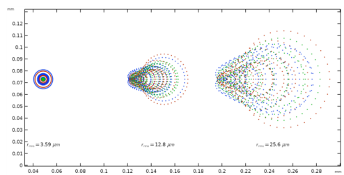
After tracing rays in 3D, you can plot the intersection points of rays with a surface using the dedicated Spot Diagram plot. This plot can only be added to a 2D Plot Group. The Spot Diagram includes many options for filtering and sorting the intersection points. It can also automatically locate a plane of best focus, and add text annotations.

The Spot Diagram can either use a Ray dataset, in which case it plots all applicable rays at the same time, or an Intersection Point 3D dataset, where the intersection points with a surface are plotted.

Use the Filters section to show or hide certain rays. This section contains check boxes for different filter criteria. You can select several of these check boxes at once, and rays will only be shown if they satisfy all of the selected criteria.

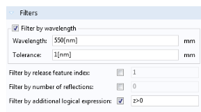
For example, you can select Filter by wavelength to hide rays of all wavelengths except a selected value; then select Filter by release feature index to only show rays that are released by a specific feature (e.g. Release from Grid 1). In many examples of cameras and telescopes in the Application Libraries, each release feature corresponds to a distinct field angle for light entering the optical system.

The check box Filter by number of reflections should only be used if you previously selected Count reflections in the physics interface Additional Variables section.

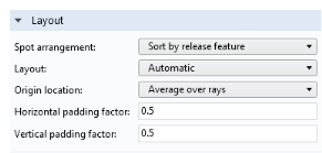
Use the Layout section to organize rays into different spots based on release feature or wavelength. If the model has multiple wavelengths or release features, this could result in an array of different spots being plotted at the same time. This section also has settings for the positioning of these different spots relative to each other in the Graphics window. For example, you can adjust the Horizontal padding factor to increase the horizontal spacing between the spots.

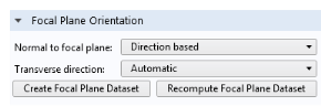
The Focal Plane Orientation section can be used to automatically locate a plane of best focus for the optical system. When you click Create Focal Plane Dataset, an Intersection Point 3D dataset will be created at a local minimum of the root mean square (rms) spot size. If the rays stop at a surface in the model and the plane of best focus is behind this surface, the automatic focal plane calculation might fail. Consider deleting the absorbing boundary, or replacing it with a Wall with the Pass through condition.

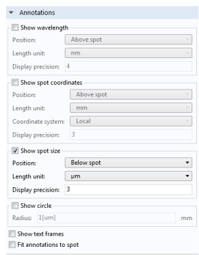
The Annotations section can add text above or below the spots in the Graphics window. These annotations can show the position, rms spot size, and wavelength (or wavelength range) of each spot. There is also an option to draw a circle in the plot, which could be used to draw the Airy disk for scale.