For the Free Molecular Flow interface when the Knudsen number is much greater than 1, collisions between gas molecules as they traverse the interior of a system can be ignored. There are two common approaches to solving the flow in this case: the Monte Carlo method (which computes the trajectories of large numbers of randomized particles through the system) and the angular coefficient method. COMSOL Multiphysics uses the angular coefficient method, which computes the molecular flow by summing the flux arriving at a surface from all other surfaces in its line of sight. The macroscopic variables in the vicinity of the surface can be derived from kinetic theory.

In many cases it is reasonable to assume that molecules are adsorbed and subsequently diffusely emitted from the surface (this is often referred to as total accommodation). In this instance, the appropriate probability density functions for emission from a surface ρ (θ, c) (SI unit: m−1s), where θ is the angle to the normal (SI unit: rad) and c is the particle speed (SI unit: ms−1), have been derived from the laws of physical gas dynamics and verified by molecular dynamics simulations (Ref. 1). A complete derivation of the probability distribution function in 2D is given in this section.

for θ in the range (−π/2, π/2) for both cylindrical (2D) and polar (3D) coordinates. In 3D the azimuthal angle φ is in the range (0, π).

Let cx and cy be the velocity components in the parallel and wall normal directions, respectively. The relationships between the velocity components in Cartesian and polar coordinates are

However, as shown in the following derivation, the interactions with the surface in the normal direction are not symmetric and do not follow a Gaussian distribution, so the probability distribution function of the molecule speed c differs from the usual 2D Maxwell distribution.

Applying Equation 3-13 to the normalization condition yields

Substituting Equation 3-12 into the modified normalization condition then yields

The functional form of that satisfies both the normalization requirement and the cosine law (Equation 3-11) is

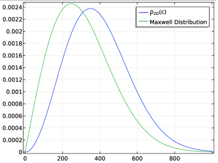
Combining Equation 3-12 and Equation 3-14 yields the probability distribution function of the speed c,

which is noticeably different from the Maxwell distribution in 2D, as shown in Figure 3-1.

Repeating the derivation of the previous section in 3D yields an analogous probability distribution function; as in 2D, the result is found to differ from the distribution function of c that would be obtained naively from the Maxwell-Boltzmann distribution. The results in both 2D and 3D are summarized below. The polar angle distribution always follows the cosine law,

based on space dimension. In 3D, the probability distribution function of the azimuthal angle φ is uniform over the interval (0, π).