|
|
|
|
•
|
When first setting up plots, it is useful to select the Only plot when requested option as some plots take a long time to render. Another trick is to use only a few rays initially.
|
|
•
|
Once the plots are set up, then before running the model (with a large number of rays), select the Recompute all plot data after solving option. Once the model has solved the plots will be rendered. This is very useful when running the model over lunch break or over night since rendering the IR plot often takes longer time than solving the model.
|
|
•
|
Before saving the model, remember to set the Save plot data list to On. Then all plots do not need to be re-rendered once the model is opened again.
|
|
1
|
|
2
|
|
3
|
Click Add.
|
|
4
|
Click Study.
|
|
5
|
|
6
|
Click Done.
|
|
1
|
|
2
|
Browse to the model’s Application Libraries folder and double-click the file small_concert_hall_geom_sequence.mph.
|
|
3
|
|
4
|
|
1
|
|
2
|
|
3
|
|
4
|
Browse to the model’s Application Libraries folder and double-click the file small_concert_hall_parameters.txt.
|
|
1
|
|
2
|
|
3
|
|
4
|
Click Browse.
|
|
5
|
Browse to the model’s Application Libraries folder and double-click the file small_concert_hall_absorption_parameters.txt.
|
|
6
|
|
7
|
Click Import.
|
|
8
|
Find the Functions subsection. In the table, enter the following settings:
|
|
9
|
Locate the Interpolation and Extrapolation section. From the Interpolation list, choose Nearest neighbor.
|
|
10
|
|
11
|
|
1
|
|
2
|
|
3
|
|
4
|
Click Browse.
|
|
5
|
Browse to the model’s Application Libraries folder and double-click the file small_concert_hall_volume_absorption.txt.
|
|
6
|
Click Import.
|
|
7
|
|
8
|
Locate the Interpolation and Extrapolation section. From the Interpolation list, choose Nearest neighbor.
|
|
9
|
|
10
|
|
1
|
|
2
|
|
3
|
In the Settings window for Variables, type Variables: Reverberation Time Estimates in the Label text field.
|
|
4
|
|
5
|
Browse to the model’s Application Libraries folder and double-click the file small_concert_hall_variables.txt.
|
|
1
|
|
2
|
|
3
|
|
4
|
|
1
|
|
2
|
|
3
|
|
4
|
|
1
|
|
2
|
|
3
|
|
4
|
|
1
|
|
2
|
|
3
|
|
4
|
|
1
|
|
2
|
|
3
|
|
4
|
|
1
|
|
2
|
|
3
|
|
4
|
|
1
|
|
2
|
|
3
|
|
4
|
|
1
|
|
2
|
|
3
|
|
4
|
Locate the Material Properties of Exterior and Unmeshed Domains section. In the cext text field, type c0.
|
|
5
|
|
6
|
|
1
|
|
2
|
|
3
|
|
1
|
|
2
|
|
3
|
|
4
|
|
5
|
|
1
|
|
2
|
|
3
|
|
4
|
|
5
|
|
1
|
|
2
|
|
3
|
|
4
|
|
5
|
|
1
|
|
2
|
|
3
|
|
4
|
|
5
|
|
1
|
|
2
|
|
3
|
|
4
|
Locate the Wall Condition section. From the Wall condition list, choose Mixed diffuse and specular reflection.
|
|
5
|
|
6
|
|
7
|
|
1
|
|
2
|
|
3
|
|
4
|
|
5
|
|
1
|
|
2
|
|
3
|
|
4
|
|
5
|
|
1
|
|
2
|
|
3
|
|
4
|
|
1
|
|
2
|
|
3
|
|
4
|
|
5
|
|
6
|
|
7
|
|
8
|
|
1
|
|
2
|
|
3
|
|
4
|
|
5
|
|
1
|
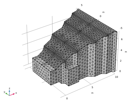
In the Model Builder window, under Component 1 (comp1) right-click Mesh 1 and choose More Operations>Free Triangular.
|
|
2
|
|
3
|
|
1
|
|
2
|
|
3
|
|
4
|
|
1
|
|
2
|
|
3
|
|
4
|
|
1
|
|
2
|
|
3
|
Click Add.
|
|
4
|
Click Range.
|
|
5
|
|
6
|
|
7
|
|
8
|
Click Replace.
|
|
9
|
|
1
|
|
2
|
|
3
|
|
1
|
|
2
|
|
3
|
|
4
|
|
1
|
|
2
|
|
3
|
|
4
|
|
1
|
|
2
|
|
3
|
|
4
|
|
5
|
|
6
|
|
7
|
|
8
|
|
1
|
|
2
|
|
3
|
|
4
|
|
5
|
|
6
|
|
7
|
|
8
|
|
9
|
Locate the Extra Time Steps section. From the Maximum number of extra time steps rendered list, choose Proportional to number of solution times.
|
|
10
|
|
1
|
|
2
|
|
3
|
|
4
|
|
1
|
|
2
|
|
3
|
|
1
|
|
2
|
In the Settings window for Group, type Group: Convergence Analysis Data Sets in the Label text field.
|
|
1
|
|
2
|
In the Settings window for Receiver 3D, type Receiver 3D - Single Band (prop = 1) in the Label text field.
|
|
3
|
|
4
|
|
5
|
|
6
|
|
7
|
|
8
|
|
9
|
|
10
|
Locate the Extra Time Steps section. From the Maximum number of extra time steps rendered list, choose Proportional to number of solution times.
|
|
1
|
|
2
|
In the Settings window for Receiver 3D, type Receiver 3D - Single Band (prop = 10) in the Label text field.
|
|
3
|
|
1
|
|
2
|
In the Settings window for Receiver 3D, type Receiver 3D - Single Band (prop = 30) in the Label text field.
|
|
3
|
|
1
|
|
2
|
In the Settings window for Receiver 3D, type Receiver 3D - Single Band (prop = 100) in the Label text field.
|
|
3
|
|
1
|
|
2
|
|
3
|
|
1
|
|
2
|
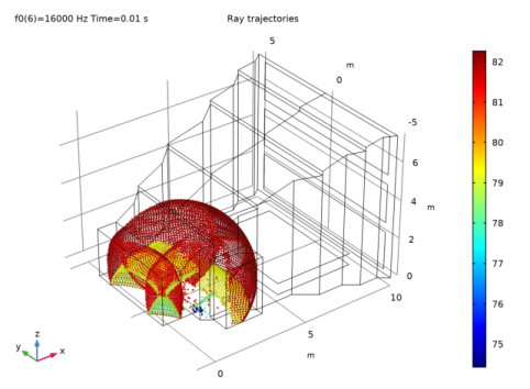
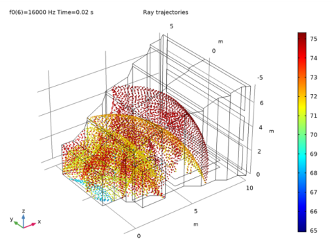
Click Plot.
|
|
1
|
|
2
|
|
3
|
|
4
|
|
1
|
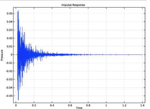
In the Model Builder window, expand the Results>Impulse Response FFT node, then click Impulse Response 1.
|
|
2
|
|
3
|
|
4
|
|
5
|
|
6
|
|
7
|
|
1
|
|
2
|
|
3
|
|
1
|
|
2
|
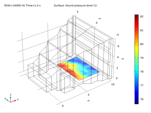
In the Settings window for Surface, click Replace Expression in the upper-right corner of the Expression section. From the menu, choose Component 1>Ray Acoustics>Accumulated variables>Wall intensity comp1.rac.wall9.spl1.Iw>rac.wall9.spl1.Lp - Sound pressure level - dB.
|
|
3
|
|
1
|
|
2
|
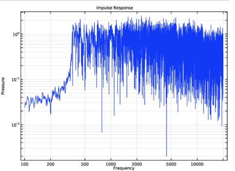
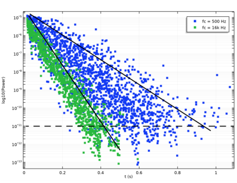
In the Settings window for 1D Plot Group, type Energetic Impulse Response (Reflectogram) in the Label text field.
|
|
3
|
|
4
|
|
5
|
|
6
|
|
7
|
In the associated text field, type log10(Power).
|
|
8
|
|
9
|
|
1
|
|
2
|
|
3
|
|
4
|
|
5
|
Click to expand the Coloring and Style section. Find the Line style subsection. From the Line list, choose None.
|
|
6
|
|
7
|
|
8
|
|
9
|
|
1
|
|
2
|
|
3
|
|
4
|
Locate the Legends section. In the table, enter the following settings:
|
|
5
|
|
1
|
|
2
|
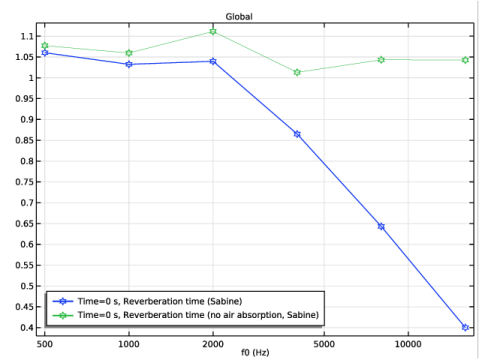
In the Settings window for 1D Plot Group, type Reverberation Time Estimates in the Label text field.
|
|
3
|
|
4
|
|
5
|
|
6
|
|
1
|
|
2
|
|
4
|
|
5
|
Click to expand the Coloring and Style section. Find the Line markers subsection. From the Marker list, choose Star.
|
|
6
|
|
7
|
|
1
|
|
2
|
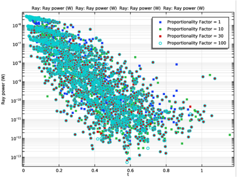
In the Settings window for 1D Plot Group, type Extra Time-Steps Convergence Analysis in the Label text field.
|
|
3
|
|
4
|
|
1
|
|
2
|
|
3
|
|
4
|
|
5
|
Locate the Coloring and Style section. Find the Line style subsection. From the Line list, choose None.
|
|
6
|
|
7
|
|
8
|
|
9
|
|
1
|
|
2
|
|
3
|
|
4
|
Locate the Legends section. In the table, enter the following settings:
|
|
1
|
|
2
|
|
3
|
|
4
|
Locate the Legends section. In the table, enter the following settings:
|
|
1
|
|
2
|
|
3
|
|
4
|
Locate the Coloring and Style section. Find the Line markers subsection. From the Marker list, choose Circle.
|
|
5
|
Locate the Legends section. In the table, enter the following settings:
|
|
6
|
|
1
|
|
2
|
In the Settings window for Evaluation Group, type Evaluation Group: Arrival Time of First Ray in the Label text field.
|
|
3
|
|
1
|
|
2
|
|
4
|
|
1
|
|
2
|
|
3
|
Click Browse.
|
|
4
|
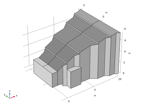
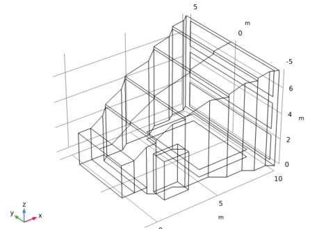
Browse to the model’s Application Libraries folder and double-click the file small_concert_hall.mphbin.
|
|
5
|
Click Import.
|
|
6
|
|
1
|
|
2
|
|
3
|
|
4
|
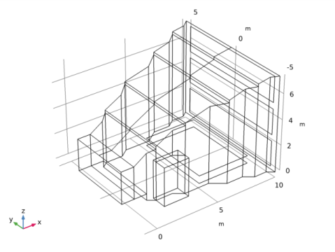
On the object imp1, select Boundaries 60–62 only.
|
|
1
|
|
2
|
|
3
|
|
4
|
On the object imp1, select Boundary 39 only.
|
|
1
|
|
2
|
|
3
|
|
4
|
On the object imp1, select Boundaries 13, 15, 29, 30, 41, 42, 49, and 50 only.
|
|
1
|
|
2
|
|
3
|
|
4
|
On the object imp1, select Boundaries 3, 8, 12, 14, 18, and 21 only.
|
|
1
|
|
2
|
|
3
|
|
4
|
On the object imp1, select Boundaries 16, 19, 20, 23, 31, and 32 only.
|
|
1
|
|
2
|
|
3
|
|
4
|
On the object imp1, select Boundaries 7, 9–11, 17, 22, 24–28, 34–37, 43–48, and 51–59 only.
|
|
1
|
|
2
|
|
3
|
|
4
|
On the object imp1, select Boundaries 1, 2, 4–6, 33, and 38 only.
|
|
1
|
|
2
|