You are viewing the documentation for an older COMSOL version. The latest version is available here.
PDF

Isotropic-Anisotropic Sample:
Elastic Wave Propagation
Introduction
This tutorial shows how to use the Elastic Waves, Time Explicit physics interface to model the propagation of elastic waves in heterogeneous anisotropic linear elastic media. The case where the material properties differ from one subdomain to another requires an special handling. Namely, the Material Discontinuity interior boundary condition (or the Continuity pair condition for assemblies) is to be explicitly imposed upon the interface between such subdomains.
In addition, the model demonstrates how to retrieve the displacements at the points of interest from the solution that contains the structural velocity and the strain.
Model Definition
A two-dimensional space is occupied by two linear elastic materials: an anisotropic material to the left of the axis x = 0 and an isotropic material to the right. The material properties are given in Table 1 (kg/m3 for the density and 1010 Pa for the stiffness). The other material parameters are c33 = c22, c13 = c23 = c12, and c44 = c55 = c66.
ρ
c11
c12
c22
c66
The elastic waves are excited by a point force applied in the y direction at the point
x0 = −2 cm, y0 = 0 cm. The source distribution in time is given by a Ricker (also known as Mexican hat) wavelet depicted in Figure 1. It has the dominant frequency f0 = 170 kHz, the time delay t0 = μs, and the amplitude of 1013 N.
The elastic 2D space is modeled as a square with the side length of 2L, L = 20 cm and the center located at (0, 0). The subdomains with the anisotropic and the isotropic properties lie to the left and to the right of the line x = 0, respectively. Four listening points are put to record the seismograms (displacement at points) at the coordinates (10.5 cm, 8 cm), (3.5 cm, 8 cm), (1.0 cm, 8 cm), and (10.5 cm, 8 cm). The model geometry layout is shown in Figure 2.
The propagation of the elastic waves in infinite space is modeled by imposing the Absorbing Layers from all four sides of the square. Combined with the Low-Reflecting Boundary condition that is imposed upon the outer boundary of the square, the Absorbing Layers ensure the reduction of the spuriously reflected waves in the physical domain.
Figure 1: A Ricker wavelet that defines the source distribution in time.
The Elastic Waves, Time Explicit interface solves for the structural velocity and the strain. The displacements can be retrieved from the velocities by solving the corresponding ordinary differential equation
In this model, this ODE is only solved at the probe points.
Figure 2: Model geometry layout.
Results and Discussion
Figure 3 shows the quantitative evolution of the waves propagating from the source at t = 30, 60, and 90 μs. One can see the round profiles of the longitudinal and the shear waves in the isotropic material on the right side. At the same time, the quasilongitudinal and the quasishear waves in the anisotropic material on the right side have the elliptic and the conical profiles, respectively. Note that the absorbing layer domains are not shown in Figure 3.
Figure 4 shows the profiles of the vertical displacement (seismograms) retrieved from the computed velocities at the probe points. The results have a good agreement in their shapes with those given in Ref. 1.
Figure 3: Velocity magnitude profiles at 30, 60, and 90 μs.
Figure 4: Seismograms at the probe points.
Notes About the COMSOL Implementation
The force load at the point (x0, y0) is modeled as a Body Load with a Total force applied to the physical domain. In theory, the load applied on the domain level must have proportional to the Dirac delta to be equivalent to a point load. That is,
One of the Dirac delta representations reads
This fact is used to approximate the point source by a domain source that has the form of a product of the temporal part and the spatial part. Here, the former is the Ricker wavelet depicted in Figure 1 and the latter is a Gaussian pulse with a relatively small extent a.
The default approximation order used in the Elastic Wave, Time Explicit interface is quartic. In this case, the maximum mesh element size that resolves the minimum wavelength λmin must not exceed λmin/1.5. The minimum wavelength is defined by the frequency content of the source, which is the Ricker wavelet here. Its frequency domain representation reads
where f0 is the dominant frequency. Although the upper cutoff frequency of the wavelet is 3f0, λmin is chosen to correspond to 2f0 in this model. This is a compromise that on one hand accounts for the greatest part of the source energy, and on the other hand does not result in a too fine mesh that would slow down the simulation and tremendously increase the model file size.
Reference
1. J. de la Puente, M. Käser, M. Dumbser and H. Igel, “An arbitrary high-order discontinuous Galerkin method for elastic waves on unstructured meshes – IV. Anisotropy”, Geophys. J. Int., vol. 169, issue 3, 2007.
Application Library path: Acoustics_Module/Elastic_Waves/isotropic_anisotropic_sample
Modeling Instructions
From the File menu, choose New.
New
In the New window, click Model Wizard.
Model Wizard
1
In the Model Wizard window, click 2D.
2
In the Select Physics tree, select Acoustics>Elastic Waves>Elastic Waves, Time Explicit (elte).
3
Click Add.
4
Click Study.
5
In the Select Study tree, select General Studies>Time Dependent.
6
Click Done.
Global Definitions
Parameters 1
1
In the Model Builder window, under Global Definitions click Parameters 1.
2
In the Settings window for Parameters, locate the Parameters section.
3
Click Load from File.
4
Create the source time function given by a Ricker wavelet.
Definitions
Analytic 1 (an1)
1
In the Home toolbar, click Functions and choose Local>Analytic.
2
In the Settings window for Analytic, type A in the Function name text field.
3
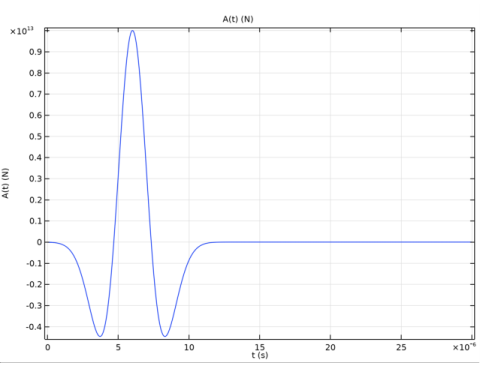
Locate the Definition section. In the Expression text field, type 1e13*(1 - 2*pi^2*f0^2*(t - t0)^2)*exp(-pi^2*f0^2*(t - t0)^2).
4
In the Arguments text field, type t.
5
Locate the Units section. In the Arguments text field, type s.
6
In the Function text field, type N.
7
Locate the Plot Parameters section. In the table, enter the following settings:
8
Click Plot.
The signal should look like the one in Figure 1
Now, create a two-dimensional Gaussian function that will be used to approximate the Dirac delta at (x0, y0).
Analytic 2 (an2)
1
In the Home toolbar, click Functions and choose Local>Analytic.
2
In the Settings window for Analytic, type G in the Function name text field.
3
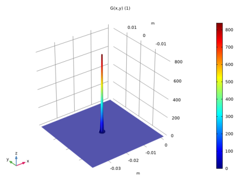
Locate the Definition section. In the Expression text field, type 1/sqrt(pi*dS)*exp(-((x - x0)^2 + (y - y0)^2)/dS).
4
In the Arguments text field, type x, y.
5
Locate the Units section. In the Arguments text field, type m.
6
In the Function text field, type 1.
7
Locate the Plot Parameters section. In the table, enter the following settings:
8
Click Plot.
Geometry 1
Square 1 (sq1)
1
In the Geometry toolbar, click Square.
2
In the Settings window for Square, locate the Size section.
3
In the Side length text field, type 2*L.
4
Locate the Position section. From the Base list, choose Center.
5
Click to expand the Layers section. Select the Layers to the left check box.
6
7
Select the Layers to the right check box.
8
Select the Layers on top check box.
Create a line segment that separates the subdomains with isotropic and anisotropic materials.
Line Segment 1 (ls1)
1
In the Geometry toolbar, click More Primitives and choose Line Segment.
2
In the Settings window for Line Segment, locate the Starting Point section.
3
From the Specify list, choose Coordinates.
4
In the y text field, type -L.
5
Locate the Endpoint section. From the Specify list, choose Coordinates.
6
In the y text field, type L.
Create four probe points for calculating the seismograms.
Point 1 (pt1)
1
In the Geometry toolbar, click Point.
2
In the Settings window for Point, locate the Point section.
3
In the x text field, type -10.5[cm] -3.5[cm] -1[cm] 10.5[cm].
4
In the y text field, type -8[cm] -8[cm] -8[cm] -8[cm].
5
Click Build All Objects.
The geometry should look like the one in Figure 2
Definitions
Explicit 1
1
In the Definitions toolbar, click Explicit.
2
In the Settings window for Explicit, locate the Input Entities section.
3
From the Geometric entity level list, choose Point.
4
5
In the Label text field, type Probe Points.
Now, set up the absorbing layers (sponge layers) used to truncate the computational domain.
Absorbing Layer 1 (ab1)
1
In the Definitions toolbar, click Absorbing Layer.
2
Setting up the materials is simpler if the correct material model is selected in the physics. Here we want to use an anisotropic material.
Elastic Waves, Time Explicit (elte)
Elastic Waves, Time Explicit Model 1
1
In the Model Builder window, under Component 1 (comp1)>Elastic Waves, Time Explicit (elte) click Elastic Waves, Time Explicit Model 1.
2
In the Settings window for Elastic Waves, Time Explicit Model, locate the Linear Elastic Material section.
3
From the Solid model list, choose Anisotropic.
Materials
Material 1 (mat1)
1
In the Model Builder window, under Component 1 (comp1) right-click Materials and choose Blank Material.
2
In the Settings window for Material, type Material Isotropic in the Label text field.
3
4
Locate the Material Contents section. In the table, enter the following settings:
Material 2 (mat2)
1
Right-click Materials and choose Blank Material.
2
In the Settings window for Material, type Material Anisotropic in the Label text field.
3
4
Locate the Material Contents section. In the table, enter the following settings:
Elastic Waves, Time Explicit (elte)
Define the force load acting at point (x0, y0) in the y-direction.
Body Load 1
1
In the Physics toolbar, click Domains and choose Body Load.
2
3
In the Settings window for Body Load, locate the Force section.
4
From the Load type list, choose Total force.
5
Specify the Ftot vector as
Low-Reflecting Boundary 1
1
In the Physics toolbar, click Boundaries and choose Low-Reflecting Boundary.
2
Impose the Material Discontinuity boundary condition upon the interface between the isotropic and anisotropic parts of the computational domain.
Material Discontinuity 1
1
In the Physics toolbar, click Boundaries and choose Material Discontinuity.
2
Mesh 1
1
In the Model Builder window, under Component 1 (comp1) click Mesh 1.
2
In the Settings window for Mesh, locate the Mesh Settings section.
3
From the Sequence type list, choose User-controlled mesh.
Size
1
In the Model Builder window, under Component 1 (comp1)>Mesh 1 click Size.
2
In the Settings window for Size, locate the Element Size section.
3
Click the Custom button.
4
Locate the Element Size Parameters section. In the Maximum element size text field, type cs_an/(2*f0)/1.5.
5
In the Minimum element size text field, type cs_an/(2*f0)/1.5.
6
Click Build All.
Study 1
1
In the Model Builder window, click Study 1.
2
In the Settings window for Study, type Study 1 - ELTE (store full solution) in the Label text field.
Step 1: Time Dependent
1
In the Model Builder window, under Study 1 - ELTE (store full solution) click Step 1: Time Dependent.
2
In the Settings window for Time Dependent, locate the Study Settings section.
3
In the Times text field, type range(0, 30[us], 90[us]).
This setting saves the solution at 30, 60, and 90 microseconds in the whole computational domain. It only influences the stored solution (and thus the file size). The internal time steps taken by the solver are automatically controlled by COMSOL to fulfill the appropriate CFL condition.
4
In the Home toolbar, click Compute.
Before plotting the results, process the dataset to display the solution in the physical domains only.
Results
Selection
1
In the Model Builder window, expand the Datasets node.
2
Right-click Study 1 - ELTE (store full solution)/Solution 1 (sol1) and choose Selection.
3
In the Settings window for Selection, locate the Geometric Entity Selection section.
4
From the Geometric entity level list, choose Domain.
5
Velocity Magnitude (elte)
1
In the Model Builder window, click Velocity Magnitude (elte).
2
In the Settings window for 2D Plot Group, locate the Data section.
3
From the Time (s) list, choose 3E-5.
Surface 1
1
In the Model Builder window, expand the Velocity Magnitude (elte) node, then click Surface 1.
2
In the Settings window for Surface, locate the Coloring and Style section.
3
From the Color table list, choose GrayScale.
4
Select the Reverse color table check box.
5
Click to expand the Range section. Select the Manual color range check box.
6
In the Maximum text field, type 5e4.
These settings will sharpen the contrast of the velocity profile.
7
In the Velocity Magnitude (elte) toolbar, click Plot.
The structural velocity profiles at the time steps chosen in Study 1 are shown in Figure 3.
Pressure (elte)
1
In the Model Builder window, click Pressure (elte).
2
In the Settings window for 2D Plot Group, locate the Data section.
3
From the Time (s) list, choose 3E-5.
4
In the Pressure (elte) toolbar, click Plot.
Next, inspect the shear and pressure wave speeds in the isotropic material and their equivalents in the anisotropic material.
2D Plot Group 3
1
In the Home toolbar, click Add Plot Group and choose 2D Plot Group.
2
In the Settings window for 2D Plot Group, type Apparent Shear Wave Speed in the Label text field.
3
Locate the Data section. From the Time (s) list, choose 3E-5.
Surface 1
1
Right-click Apparent Shear Wave Speed and choose Surface.
2
In the Settings window for Surface, locate the Expression section.
3
In the Expression text field, type elte.cs.
4
In the Apparent Shear Wave Speed toolbar, click Plot.
Apparent Shear Wave Speed 1
1
In the Model Builder window, right-click Apparent Shear Wave Speed and choose Duplicate.
2
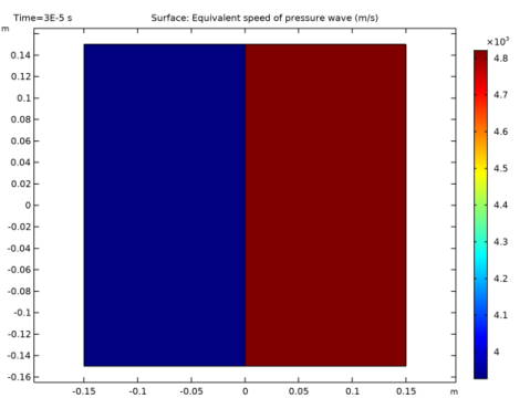
In the Settings window for 2D Plot Group, type Apparent Pressure Wave Speed in the Label text field.
Surface 1
1
In the Model Builder window, expand the Results>Apparent Pressure Wave Speed node, then click Surface 1.
2
In the Settings window for Surface, locate the Expression section.
3
In the Expression text field, type elte.cp.
4
In the Apparent Pressure Wave Speed toolbar, click Plot.
Set up an extra study to compute the seismograms at the probe points.
Add Study
1
In the Home toolbar, click Add Study to open the Add Study window.
2
Go to the Add Study window.
3
Find the Studies subsection. In the Select Study tree, select General Studies>Time Dependent.
4
Click Add Study in the window toolbar.
Study 2
1
In the Model Builder window, click Study 2.
2
In the Settings window for Study, locate the Study Settings section.
3
Clear the Generate default plots check box.
4
In the Label text field, type Study 2 - ELTE (store at points).
Step 1: Time Dependent
1
In the Model Builder window, under Study 2 - ELTE (store at points) click Step 1: Time Dependent.
2
In the Settings window for Time Dependent, locate the Study Settings section.
3
In the Times text field, type range(0, t0/20, 17*t0).
4
Click to expand the Values of Dependent Variables section. Find the Store fields in output subsection. From the Settings list, choose For selections.
5
Under Selections, click Add.
6
In the Add dialog box, select Probe Points in the Selections list.
7
With these settings, a finer time resolution is used, but the solution is only stored at the probe points. This will reduce the size of the model file.
8
In the Home toolbar, click Compute.
Next, add an auxiliary ODE to retrieve the displacements from the velocities computed in the previous study. Here, we will be interested in the y-components of the corresponding vector fields only.
Add Physics
1
In the Home toolbar, click Add Physics to open the Add Physics window.
2
Go to the Add Physics window.
3
In the tree, select Mathematics>ODE and DAE Interfaces>Point ODEs and DAEs (pode).
4
Find the Physics interfaces in study subsection. In the table, enter the following settings:
5
Click Add to Selection in the window toolbar.
Point ODEs and DAEs (pode)
1
In the Settings window for Point ODEs and DAEs, locate the Point Selection section.
2
From the Selection list, choose Probe Points.
3
Locate the Units section. Click Select Dependent Variable Quantity.
4
In the Physical Quantity dialog box, type id:displacement in the text field.
5
Click Filter.
6
In the tree, select General>Displacement (m).
7
8
In the Settings window for Point ODEs and DAEs, locate the Units section.
9
Click Select Source Term Quantity.
10
In the Physical Quantity dialog box, type id:velocity in the text field.
11
Click Filter.
12
In the tree, select General>Velocity (m/s).
13
14
In the Settings window for Point ODEs and DAEs, click to expand the Dependent Variables section.
15
In the Field name text field, type uy.
16
In the Dependent variables table, enter the following settings:
Distributed ODE 1
1
In the Model Builder window, under Component 1 (comp1)>Point ODEs and DAEs (pode) click Distributed ODE 1.
2
In the Settings window for Distributed ODE, locate the Source Term section.
3
In the f text field, type vy.
4
In the Home toolbar, click Add Study to close the Add Study window.
Add Study
1
In the Home toolbar, click Add Study to open the Add Study window.
2
Go to the Add Study window.
3
Find the Physics interfaces in study subsection. In the table, enter the following settings:
4
Find the Studies subsection. In the Select Study tree, select General Studies>Time Dependent.
5
Click Add Study in the window toolbar.
6
In the Home toolbar, click Add Study to close the Add Study window.
Study 3
1
In the Model Builder window, click Study 3.
2
In the Settings window for Study, type Study 3 - Displacement (ODE) in the Label text field.
3
Locate the Study Settings section. Clear the Generate default plots check box.
Use the same time interval as in Study 2.
Step 1: Time Dependent
1
In the Model Builder window, under Study 3 - Displacement (ODE) click Step 1: Time Dependent.
2
In the Settings window for Time Dependent, locate the Study Settings section.
3
In the Times text field, type range(0, t0/20, 17*t0).
4
Locate the Values of Dependent Variables section. Find the Values of variables not solved for subsection. From the Settings list, choose User controlled.
5
From the Method list, choose Solution.
6
From the Study list, choose Study 2 - ELTE (store at points), Time Dependent.
7
From the Time (s) list, choose All.
Modify the solver to the one appropriate for solving wave problems. This is the same default when e.g. solving a transient pressure acoustics model.
Solution 3 (sol3)
1
In the Study toolbar, click Show Default Solver.
2
In the Model Builder window, expand the Solution 3 (sol3) node, then click Time-Dependent Solver 1.
3
In the Settings window for Time-Dependent Solver, click to expand the Time Stepping section.
4
From the Method list, choose Generalized alpha.
5
From the Steps taken by solver list, choose Manual.
6
In the Time step text field, type 1/(60*f0).
7
In the Study toolbar, click Compute.
Now, plot the computed seismograms at the probe points. The results should look like the ones in Figure 4.
Results
1D Plot Group 5
1
In the Home toolbar, click Add Plot Group and choose 1D Plot Group.
2
In the Settings window for 1D Plot Group, type Displacement in (x,y) = (-10.5 cm, -8 cm) in the Label text field.
3
Locate the Data section. From the Dataset list, choose Study 3 - Displacement (ODE)/Solution 3 (sol3).
4
Click to expand the Title section. From the Title type list, choose Manual.
5
In the Title text area, type Displacement, y-component (m).
6
Locate the Plot Settings section. Select the y-axis label check box.
7
In the associated text field, type Displacement, y-component (m).
Point Graph 1
1
In the Displacement in (x,y) = (-10.5 cm, -8 cm) toolbar, click Point Graph.
2
3
In the Settings window for Point Graph, locate the y-Axis Data section.
4
In the Expression text field, type uy.
5
In the Displacement in (x,y) = (-10.5 cm, -8 cm) toolbar, click Plot.
Displacement in (x,y) = (-10.5 cm, -8 cm) 1
1
In the Model Builder window, right-click Displacement in (x,y) = (-10.5 cm, -8 cm) and choose Duplicate.
2
In the Settings window for 1D Plot Group, type Displacement in (x,y) = (-3.5 cm, -8 cm) in the Label text field.
Point Graph 1
1
In the Model Builder window, expand the Results>Displacement in (x,y) = (-3.5 cm, -8 cm) node, then click Point Graph 1.
2
In the Settings window for Point Graph, locate the Selection section.
3
Click Clear Selection.
4
5
In the Displacement in (x,y) = (-3.5 cm, -8 cm) toolbar, click Plot.
Generate the seismograms at the remaining probe points by repeating the previous instructions.