PDF

Doppler Shift
Introduction
You can notice the Doppler effect when an ambulance or a fire engine passes by with its sirens blaring. The siren’s pitch suddenly drops the moment the ambulance starts to move away from you. Another effect you can hear is how the siren’s sound suddenly becomes markedly quieter as soon as the ambulance passes.
In this example, the observer and air are at rest while the sound source, the ambulance, moves with the speed V. This gives the same effect as if the sound source were at rest and the observer and air were moving at the same speed but in the opposite direction.
Model Definition
This is an axisymmetric problem with a point source at rest at the origin, (rz) = (00), emitting spherical sound waves with the frequency f = 100 Hz. The surrounding air moves at V = 50 m/s (180 km/h or roughly 112 miles/hour) in the negative z direction. With this setup, the rz-plane is the horizontal plane at the level of the source and the observer, and the effects of reflections at the ground are neglected.
Assume, furthermore, that the observer stands 1 m from where the ambulance passes by. In the model geometry, this situation amounts to the observer moving with the flow along the line r = 1.
The boundary conditions are absorbing because there is no physical boundary around the source. This is modeled using perfectly matched layers.
Results and Discussion
The acoustic wavelength decreases for a wavefront moving in the opposite direction of the airflow. This situation corresponds to the approach stage of the ambulance, which, for the stationary observer on the ground, implies a perceived frequency that is higher than the nominal source frequency f. Conversely, the wavelength increases and the perceived frequency decreases when the acoustic wave moves with the flow during the departing stage. These two stages correspond, respectively, to the solid and dashed curves in Figure 1.
Figure 1: The x-axis represents the distance between the ambulance and the point where it passes the observer. The solid line shows the pressure perceived by the observer as the ambulance is moving toward it. The dashed line shows the pressure as the ambulance is moving away from the observer.
An inspection of Figure 1 also shows that the amplitude drops off at a faster rate when the ambulance is moving away from the observer than when it is moving toward it. This effect is also visible in Figure 2 and Figure 3, which both show the sound pressure level.
Figure 2: Sound pressure level around the point source, represented by colors and contour lines. Note how the outermost contour runs from well inside the physical domain to the PML, showing that the sound is greater below than above the source.
Figure 3: Sound pressure level at the observer’s position during the ambulance’s approach (solid, blue line) and departing (dashed, green line) versus distance from the position (r, z) = (1 m, 0)(where the observer-ambulance distance is the smallest).
Application Library path: Acoustics_Module/Aeroacoustics_and_Noise/doppler_shift
Modeling Instructions
From the File menu, choose New.
New
In the New window, click  Model Wizard.
Model Wizard
1
In the Model Wizard window, click  2D Axisymmetric.
2
In the Select Physics tree, select Acoustics>Aeroacoustics>Linearized Potential Flow, Frequency Domain (ae).
3
Click Add.
4
Click  Study.
5
In the Select Study tree, select General Studies>Frequency Domain.
6
Global Definitions
Define parameters for the background flow conditions, the signal frequency, and the geometry.
Parameters 1
1
In the Model Builder window, under Global Definitions click Parameters 1.
2
In the Settings window for Parameters, locate the Parameters section.
3
Geometry 1
Circle 1 (c1)
1
In the Geometry toolbar, click  Circle.
2
In the Settings window for Circle, locate the Size and Shape section.
3
In the Radius text field, type R0.
4
In the Sector angle text field, type 180.
5
Locate the Rotation Angle section. In the Rotation text field, type -90.
6
Click to expand the Layers section. In the table, enter the following settings:
Point 1 (pt1)
1
In the Geometry toolbar, click  Point.
2
Click  Build All Objects.
Add Material
1
In the Home toolbar, click  Add Material to open the Add Material window.
2
Go to the Add Material window.
3
4
Click Add to Component in the window toolbar.
5
In the Home toolbar, click  Add Material to close the Add Material window.
Definitions
Perfectly Matched Layer 1 (pml1)
1
In the Definitions toolbar, click  Perfectly Matched Layer.
2
Linearized Potential Flow, Frequency Domain (ae)
Linearized Potential Flow Model 1
1
In the Model Builder window, under Component 1 (comp1)>Linearized Potential Flow, Frequency Domain (ae) click Linearized Potential Flow Model 1.
2
In the Settings window for Linearized Potential Flow Model, locate the Linearized Potential Flow Model section.
3
Specify the V vector as
Mass Flow Point Source 1
1
In the Physics toolbar, click  Points and choose Mass Flow Point Source.
2
3
In the Settings window for Mass Flow Point Source, locate the Mass Flow Point Source section.
4
In the m text field, type 1e-4.
Now, set up a mesh for the model. The maximal mesh size is dictated by the shortest wavelength in the model divided by 6. In the PML region, use a mapped mesh with 8 layers.
Mesh 1
Free Triangular 1
1
In the Model Builder window, under Component 1 (comp1) right-click Mesh 1 and choose Free Triangular.
2
In the Settings window for Free Triangular, locate the Domain Selection section.
3
From the Geometric entity level list, choose Domain.
4
Size
1
In the Model Builder window, click Size.
2
In the Settings window for Size, locate the Element Size section.
3
Click the Custom button.
4
Locate the Element Size Parameters section. In the Maximum element size text field, type (343[m/s]-V)/f0/6.
5
Click  Build All.
Mapped 1
In the Model Builder window, right-click Mesh 1 and choose Mapped.
Distribution 1
1
In the Model Builder window, right-click Mapped 1 and choose Distribution.
2
3
In the Settings window for Distribution, locate the Distribution section.
4
In the Number of elements text field, type 8.
5
Click  Build All.
Study 1
Step 1: Frequency Domain
1
In the Model Builder window, under Study 1 click Step 1: Frequency Domain.
2
In the Settings window for Frequency Domain, locate the Study Settings section.
3
In the Frequencies text field, type f0.
4
In the Home toolbar, click  Compute.
Results
The default plot groups contain plots of the pressure and the sound pressure level, in 2D and 3D.
Sound Pressure Level, 3D (ae)
1
Click the  Zoom Extents button in the Graphics toolbar.
2
In the Model Builder window, under Results click Sound Pressure Level, 3D (ae).
3
In the Sound Pressure Level, 3D (ae) toolbar, click  Plot.
Contour 1
1
Right-click Sound Pressure Level, 3D (ae) and choose Contour.
2
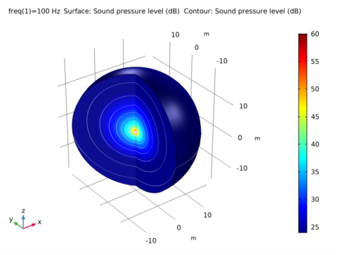
In the Settings window for Contour, click Replace Expression in the upper-right corner of the Expression section. From the menu, choose Component 1>Linearized Potential Flow, Frequency Domain>Pressure and sound pressure level>ae.Lp - Sound pressure level - dB.
3
Locate the Coloring and Style section. From the Coloring list, choose Uniform.
4
From the Color list, choose White.
5
Clear the Color legend check box.
6
In the Sound Pressure Level, 3D (ae) toolbar, click  Plot.
The plot is now dominated by the roughly 50 dB losses in the PML. To see only the physical domain, make a selection as follows.
Study 1/Solution 1 (sol1)
In the Model Builder window, expand the Results>Datasets node, then click Study 1/Solution 1 (sol1).
Selection
1
In the Results toolbar, click  Attributes and choose Selection.
2
In the Settings window for Selection, locate the Geometric Entity Selection section.
3
From the Geometric entity level list, choose Domain.
4
Sound Pressure Level, 3D (ae)
Removing the PML from the visualization moves the bias in the color scale toward the value in the source point. Mathematically, the pressure in the vicinity of this point is inversely proportional to the distance from the point. In the point itself, this means an infinitely high pressure. The discretization results in a finite but completely mesh-dependent value (the finer the mesh, the higher the pressure). The flow from the point however is well-defined and results in a converging pressure distribution at any finite distance away from the point. To suppress the highest values and get a better picture of the sound pressure level distribution, you can set the plot range manually.
Surface
1
In the Model Builder window, click Surface.
2
In the Settings window for Surface, click to expand the Range section.
3
Select the Manual color range check box.
4
In the Minimum text field, type 24.
5
In the Maximum text field, type 60.
6
In the Sound Pressure Level, 3D (ae) toolbar, click  Plot.
7
Click the  Zoom Extents button in the Graphics toolbar.
In order to recreate the line plots in the Results and Discussion section, you first need to create two cut lines, one going up and one going down from the starting point 1 m out from the source.
Cut Line 2D 1
1
In the Results toolbar, click  Cut Line 2D.
2
In the Settings window for Cut Line 2D, locate the Line Data section.
3
In row Point 1, set R to 1 and z to 0.
4
In row Point 2, set R to 1 and z to 8.
5
Cut Line 2D 2
1
In the Results toolbar, click  Cut Line 2D.
2
In the Settings window for Cut Line 2D, locate the Line Data section.
3
In row Point 1, set R to 1 and z to 0.
4
In row Point 2, set R to 1 and z to -8.
5
With the cut lines defined, create a 1D plot group for the first plot.
Pressure on Cut Lines
1
In the Results toolbar, click  1D Plot Group.
2
In the Settings window for 1D Plot Group, type Pressure on Cut Lines in the Label text field.
3
Click to expand the Title section. From the Title type list, choose Manual.
4
In the Title text area, type Pressure.
5
Locate the Plot Settings section. Select the x-axis label check box.
6
Line Graph 1
1
Right-click Pressure on Cut Lines and choose Line Graph.
2
In the Settings window for Line Graph, locate the Data section.
3
From the Dataset list, choose Cut Line 2D 1.
4
Click Replace Expression in the upper-right corner of the y-axis data section. From the menu, choose Component 1>Linearized Potential Flow, Frequency Domain>Pressure and sound pressure level>ae.p - Pressure - Pa.
5
Click to expand the Legends section.
Line Graph 2
1
Right-click Line Graph 1 and choose Duplicate.
2
In the Settings window for Line Graph, locate the Data section.
3
From the Dataset list, choose Cut Line 2D 2.
4
Click to expand the Coloring and Style section. Find the Line style subsection. From the Line list, choose Dashed.
Add legends to the plot.
Line Graph 1
1
In the Model Builder window, click Line Graph 1.
2
In the Settings window for Line Graph, locate the Legends section.
3
Select the Show legends check box.
4
From the Legends list, choose Manual.
5
Line Graph 2
1
In the Model Builder window, click Line Graph 2.
2
In the Settings window for Line Graph, locate the Legends section.
3
Select the Show legends check box.
4
From the Legends list, choose Manual.
5
Create another plot group for the second line plot.
6
In the Pressure on Cut Lines toolbar, click  Plot.
SPL on Cut Lines
1
In the Home toolbar, click  Add Plot Group and choose 1D Plot Group.
2
In the Settings window for 1D Plot Group, type SPL on Cut Lines in the Label text field.
3
Locate the Title section. From the Title type list, choose Manual.
4
In the Title text area, type Sound Pressure Level.
5
Locate the Plot Settings section. Select the x-axis label check box.
6
7
Select the y-axis label check box.
8
In the associated text field, type Sound pressure level (dB).
Line Graph 1
1
Right-click SPL on Cut Lines and choose Line Graph.
2
In the Settings window for Line Graph, locate the Data section.
3
From the Dataset list, choose Cut Line 2D 1.
4
Click Replace Expression in the upper-right corner of the y-axis data section. From the menu, choose Component 1>Linearized Potential Flow, Frequency Domain>Pressure and sound pressure level>ae.Lp - Sound pressure level - dB.
Line Graph 2
1
Right-click Line Graph 1 and choose Duplicate.
2
In the Settings window for Line Graph, locate the Data section.
3
From the Dataset list, choose Cut Line 2D 2.
4
Locate the Coloring and Style section. Find the Line style subsection. From the Line list, choose Dashed.
Line Graph 1
1
In the Model Builder window, click Line Graph 1.
2
In the Settings window for Line Graph, locate the Legends section.
3
Select the Show legends check box.
4
From the Legends list, choose Manual.
5
Line Graph 2
1
In the Model Builder window, click Line Graph 2.
2
In the Settings window for Line Graph, locate the Legends section.
3
Select the Show legends check box.
4
From the Legends list, choose Manual.
5
6
In the SPL on Cut Lines toolbar, click  Plot.