|
|
|
|
1
|
|
2
|
Click Done.
|
|
1
|
|
2
|
Browse to the model’s Application Libraries folder and double-click the file acoustics_pipe_system_geom_sequence.mph.
|
|
3
|
|
1
|
|
2
|
|
1
|
|
2
|
|
3
|
|
4
|
Browse to the model’s Application Libraries folder and double-click the file acoustics_pipe_system_parameters.txt.
|
|
1
|
|
2
|
|
3
|
|
4
|
|
5
|
|
1
|
|
2
|
|
3
|
|
4
|
|
5
|
|
6
|
|
7
|
|
8
|
|
9
|
Click Plot.
|
|
1
|
|
2
|
|
3
|
|
1
|
|
2
|
|
3
|
|
1
|
|
2
|
|
3
|
|
4
|
|
5
|
|
1
|
|
2
|
|
3
|
|
4
|
|
1
|
|
2
|
|
3
|
|
1
|
|
2
|
|
3
|
|
4
|
|
5
|
|
6
|
|
7
|
|
8
|
|
9
|
|
10
|
|
11
|
|
12
|
|
1
|
|
2
|
|
3
|
|
4
|
|
1
|
In the Model Builder window, under Component 1 (comp1)>Pipe Acoustics, Transient (patd) click Pipe Properties 1.
|
|
2
|
|
3
|
From the list, choose Circular.
|
|
4
|
|
1
|
|
3
|
|
4
|
From the list, choose Circular.
|
|
5
|
|
1
|
|
2
|
|
3
|
|
1
|
|
3
|
|
4
|
Specify the F vector as
|
|
1
|
|
2
|
In the Settings window for Pressure Acoustics, Transient, locate the Transient Solver Settings section.
|
|
3
|
|
1
|
In the Model Builder window, under Component 1 (comp1) click Pressure Acoustics, Boundary Mode (acbm).
|
|
2
|
In the Settings window for Pressure Acoustics, Boundary Mode, locate the Boundary Selection section.
|
|
3
|
|
1
|
In the Model Builder window, under Component 1 (comp1) click Pipe Acoustics, Frequency Domain (pafd).
|
|
2
|
|
3
|
|
1
|
In the Model Builder window, under Component 1 (comp1)>Pipe Acoustics, Frequency Domain (pafd) click Pipe Properties 1.
|
|
2
|
|
3
|
From the list, choose Circular.
|
|
4
|
|
1
|
|
3
|
|
4
|
From the list, choose Circular.
|
|
5
|
|
1
|
|
2
|
|
3
|
|
1
|
|
3
|
|
4
|
Specify the F vector as
|
|
1
|
In the Physics toolbar, click Multiphysics Couplings and choose Global>Acoustic-Pipe Acoustic Connection.
|
|
2
|
In the Settings window for Acoustic-Pipe Acoustic Connection, locate the Coupled Interfaces section.
|
|
3
|
|
4
|
|
1
|
|
2
|
|
3
|
|
1
|
|
2
|
|
3
|
Click the Custom button.
|
|
4
|
Locate the Element Size Parameters section. In the Maximum element size text field, type min(lam0/12,Di/2).
|
|
5
|
|
6
|
|
1
|
|
2
|
|
3
|
|
1
|
|
1
|
|
2
|
|
3
|
Click the Custom button.
|
|
4
|
|
5
|
|
6
|
|
7
|
|
8
|
|
1
|
|
2
|
Find the Studies subsection. In the Select Study tree, select Preset Studies for Some Physics Interfaces>Time Dependent.
|
|
3
|
|
4
|
|
5
|
|
6
|
|
1
|
|
2
|
|
3
|
|
4
|
|
5
|
|
6
|
|
7
|
|
1
|
|
2
|
|
3
|
|
4
|
|
5
|
Find the Studies subsection. In the Select Study tree, select Preset Studies for Selected Physics Interfaces>Mode Analysis.
|
|
6
|
|
1
|
|
2
|
|
3
|
|
1
|
|
2
|
|
3
|
|
4
|
|
6
|
|
7
|
|
1
|
|
2
|
|
3
|
|
4
|
|
5
|
|
1
|
|
2
|
In the Settings window for Study, type Study 3 - Pipe System Frequency Domain in the Label text field.
|
|
3
|
|
1
|
In the Model Builder window, under Study 3 - Pipe System Frequency Domain click Step 1: Frequency Domain.
|
|
2
|
|
3
|
|
4
|
|
1
|
|
2
|
|
3
|
|
4
|
|
5
|
|
6
|
Click OK.
|
|
1
|
|
2
|
|
3
|
|
4
|
|
5
|
|
6
|
|
7
|
|
8
|
|
9
|
|
1
|
|
2
|
|
3
|
|
4
|
|
5
|
|
6
|
|
7
|
|
8
|
|
9
|
|
10
|
|
1
|
|
2
|
|
3
|
|
4
|
|
5
|
|
6
|
Select the Description check box.
|
|
1
|
|
2
|
|
3
|
|
4
|
|
1
|
|
2
|
|
3
|
|
4
|
|
5
|
|
1
|
|
2
|
|
3
|
|
4
|
|
1
|
|
2
|
|
3
|
|
4
|
|
5
|
|
1
|
|
2
|
|
3
|
|
4
|
|
5
|
|
6
|
|
1
|
|
2
|
|
3
|
|
4
|
|
5
|
|
6
|
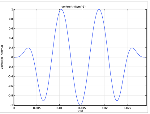
In the associated text field, type Time (s).
|
|
7
|
|
8
|
In the associated text field, type Pressure (Pa).
|
|
9
|
|
1
|
|
2
|
|
4
|
|
5
|
|
1
|
|
2
|
|
4
|
|
5
|
|
6
|
|
1
|
|
2
|
|
4
|
|
5
|
|
6
|
|
8
|
|
1
|
|
2
|
In the Settings window for 2D Plot Group, type Mode analysis pressure (acbm) in the Label text field.
|
|
1
|
|
2
|
|
3
|
|
4
|
|
5
|
|
6
|
|
1
|
|
2
|
|
3
|
Locate the Data section. From the Dataset list, choose Study 3 - Pipe System Frequency Domain/Solution 3 (sol3).
|
|
4
|
|
5
|
|
6
|
|
7
|
|
1
|
|
2
|
|
3
|
|
4
|
|
5
|
|
6
|
|
7
|
|
8
|
|
1
|
|
2
|
|
3
|
|
4
|
|
5
|
|
6
|
|
1
|
|
2
|
|
3
|
|
4
|
|
1
|
|
2
|
|
3
|
|
4
|
|
5
|
|
6
|
|
1
|
|
2
|
Click Done.
|
|
1
|
|
2
|
|
3
|
|
4
|
Browse to the model’s Application Libraries folder and double-click the file acoustics_pipe_system_geom_sequence_parameters.txt.
|
|
5
|
|
1
|
|
2
|
|
3
|
|
4
|
|
5
|
|
6
|
|
7
|
|
1
|
|
2
|
|
3
|
|
4
|
|
5
|
|
6
|
|
7
|
|
1
|
|
2
|
|
3
|
|
4
|
|
5
|
|
6
|
|
7
|
|
1
|
|
2
|
|
3
|
|
4
|
|
5
|
|
6
|
|
7
|
|
8
|
|
1
|
|
2
|
|
3
|
|
1
|
|
2
|
|
3
|
|
4
|
|
5
|
|
6
|
|
7
|
|
8
|
|
9
|
|
1
|
|
2
|
|
3
|
|
4
|
|
5
|
|
6
|
|
1
|
|
2
|
|
3
|
|
4
|
|
5
|
|
6
|
|
7
|
|
8
|
|
1
|
|
2
|
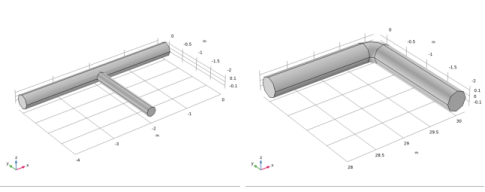
On the object cyl3, select Boundary 4 only.
|
|
3
|
|
4
|
Click the Angles button.
|
|
5
|
|
6
|
|
7
|
Locate the Revolution Axis section. Find the Point on the revolution axis subsection. In the yw text field, type -rbend-Di/2.
|
|
8
|
|
9
|
|
10
|
|
1
|
|
2
|
|
3
|
|
4
|
|
5
|
|
6
|
|
7
|
|
8
|
|
1
|
|
2
|
|
3
|
|
4
|
|
5
|
|
6
|
|
7
|
|
8
|
|
9
|
|
10
|