Acoustic Cloaking

In the tree, select .

The geometry of this model is simple but a bit repetitive to create, due to the large number of circles involved. You will therefore import it inserting a sequence from the geometry file. The instructions to the geometry can be found in the appendix at the end of this document.

Geometry 1

In the toolbar, click .

Browse to the model’s Application Libraries folder and double-click the file acoustic_cloaking_geom_sequence.mph.

In the toolbar, click .

Click the button in the toolbar.

The geometry should look like that in Figure 1.

The file you have just imported contains a few parameters that are used to generate the geometry. Now proceed to add some additional parameters that will be used in the analysis.

Global Definitions

Parameters 1

In the window, under click .

In the window for , locate the section.

The material properties in the cloaking involve dependencies on the inner and outer radius, the local distance from the center, and the properties of the surrounding background fluid. It is convenient to define these expressions as variables.


Name	Expression	Value	Description
rhob	1.25[kg/m^3]	1.25 kg/m³	Density, background material
cb	343[m/s]	343 m/s	Speed of sound, background material
f0	300[Hz]	300 Hz	Frequency of the analysis
lam0	cb/f0	1.1433 m	Wavelength

Definitions

Cylindrical System 2 (sys2)

In the toolbar, click and choose .

In the window for , locate the section.

Find the subsection. In the table, enter the following settings:


x (m)	y (m)
x1	y1

Variables 1

In the window, right-click and choose .

In the window for , type Radial Coordinate: Homogenized Cloak in the text field.

Locate the section. From the list, choose .

From the list, choose .

Locate the section. In the table, enter the following settings:


Name	Expression	Unit	Description
r	sys2.r	m	Radial Coordinate

Variables 2

Right-click and choose .

In the window for , type Radial Coordinate: 50 Layer Cloak in the text field.

Locate the section. From the list, choose .

From the list, choose .

Locate the section. In the table, enter the following settings:


Name	Expression	Unit	Description
r	sqrt((x-x3)^2+(y-y3)^2)	m	Radial Coordinate

Variables 3

Right-click and choose .

In the window for , type Radial Coordinate: 20 Layer Cloak in the text field.

Locate the section. From the list, choose .

From the list, choose .

Locate the section. In the table, enter the following settings:


Name	Expression	Unit	Description
r	sqrt((x-x4)^2+(y-y4)^2)	m	Radial Coordinate

Variables 4

In the toolbar, click .

In the window for , type Variables: Acoustic Cloak Data in the text field.

Locate the section. From the list, choose .

From the list, choose .

Locate the section. In the table, enter the following settings:


Name	Expression	Unit	Description
rho1	rhob(r+sqrt(2r*R1-R1^2))/(r-R1)	kg/m³	Density, Material 1
c1	cb(R2-R1)/R2r/(r-R1)	m/s	Speed of sound, Material 1
rho2	rhob^2/rho1	kg/m³	Density, Material 2
c2	c1	m/s	Speed of sound, Material 2
K1	rho1*c1^2	Pa	Bulk modulus, Material 2
K2	rho2*c2^2	Pa	Bulk modulus, Material 2
K	2K1K2/(K1+K2)	Pa	Effective bulk modulus
rho_tangential	2rho1rho2/(rho1+rho2)	kg/m³	Density along layers
rho_normal	(rho1+rho2)/2	kg/m³	Density perpendicular to the layers

Now, proceed to add the materials. Material 1 and Material 2 are the two materials with varying properties that will be used in the layers to create an acoustic cloak. The homogenized material is an anisotropic material which properties also vary with thickness and are equivalent to a model with a large number of layers.

Materials

Material 1 (mat1)

In the window, under right-click and choose .

In the window for , type Air in the text field.

Locate the section. From the list, choose .

Locate the section. In the table, enter the following settings:


Property	Variable	Value	Unit	Property group
Density	rho	rhob	kg/m³	Basic
Speed of sound	c	cb	m/s	Basic

Material 2 (mat2)

Right-click and choose .

In the window for , type Material 1 in the text field.

Locate the section. From the list, choose .

Locate the section. In the table, enter the following settings:


Property	Variable	Value	Unit	Property group
Density	rho	rho1	kg/m³	Basic
Speed of sound	c	c1	m/s	Basic

Material 3 (mat3)

Right-click and choose .

In the window for , type Material 2 in the text field.

Locate the section. From the list, choose .

Locate the section. In the table, enter the following settings:


Property	Variable	Value	Unit	Property group
Density	rho	rho2	kg/m³	Basic
Speed of sound	c	c2	m/s	Basic

Material 4 (mat4)

Right-click and choose .

In the window for , type Homogenized Material in the text field.

Locate the section. From the list, choose .

Click to expand the section. In the tree, select .

Click .

In the tree, select .

In the window for , locate the section.

The homogenized material has a diagonal density matrix with terms that change value with the radius. The bulk modulus also varies with the radius.


Property	Variable	Value	Unit	Property group
Effective density	{rho_eff11, rho_eff22, rho_eff33} ; rho_effij = 0	{rho_normal,rho_tangential,rho_tangential}	kg/m³	Anisotropic acoustics model
Effective bulk modulus	K_eff	K	Pa	Anisotropic acoustics model
Density	rho		kg/m³	Basic
Speed of sound	c		m/s	Basic

Now, proceed to activate the that will give you access to the feature. This feature allows you to compute the speed of sound in the anisotropic material as a function of the density matrix and the bulk modulus.

Definitions

Click the button in the toolbar.

In the dialog box, select in the tree.

In the tree, select the check box for the node .

Matrix Diagonalization 1 (matdiag1)

In the toolbar, click and choose .

In the window for , locate the section.

From the list, choose .

Select Domain 4 only.

Locate the section. In the table, enter the following settings:


acpr.rho_eff_invxx*K	acpr.rho_eff_invxy*K	acpr.rho_eff_invxz*K
acpr.rho_eff_invxy*K	acpr.rho_eff_invyy*K	acpr.rho_eff_invyz*K
acpr.rho_eff_invxz*K	acpr.rho_eff_invxy*K	acpr.rho_eff_invzz*K

These terms represent the inverse of the effective density matrix times the bulk modulus. The square root of the eigenvalues of this matrix will give you the speed of sound in the principal directions.

Pressure Acoustics, Frequency Domain (acpr)

Group 1

In the window, under right-click and choose .

In the window for , type Homogenized model in the text field.

The outer boundaries need a radiation condition to make sure that no waves are reflected at this interface.

Cylindrical Wave Radiation 1

Right-click and choose .

Select Boundary 154 only.

In the window, click .

In the window for , locate the section.

Specify the r0 vector as


x1	x
y1	y

Homogenized model

Now, proceed to add a for each of the geometries. The field is a plane wave propagating in the -direction. The phase of this field is updated on each of the domains to make sure that the incident acoustic field is the same in all the domains.

Background Pressure Field 1

In the toolbar, click and choose .

In the window for , locate the section.

From the list, choose .

Locate the section. In the p0 text field, type 1.

From the c list, choose .

From the list, choose .

In the φ text field, type acpr.bpf1.k*x1.

Symmetry 1

In the toolbar, click and choose .

In the window for , locate the section.

From the list, choose .

Anisotropic Acoustics 1

In the toolbar, click and choose .

Select Domain 4 only.

In the window for , locate the section.

From the list, choose .

Group 2

In the window, right-click and choose .

In the window for , type No Cloak Model in the text field.

Cylindrical Wave Radiation 2

In the toolbar, click and choose .

Select Boundary 209 only.

In the window for , locate the section.

Specify the r0 vector as


x2	x
y2	y

Background Pressure Field 2

In the toolbar, click and choose .

In the window for , locate the section.

From the list, choose .

Locate the section. In the p0 text field, type 1.

From the c list, choose .

In the φ text field, type acpr.bpf2.k*x2.

Symmetry 2

In the toolbar, click and choose .

In the window for , locate the section.

From the list, choose .

Group 3

Right-click and choose .

In the window for , type 50 Layer Cloak Model in the text field.

Cylindrical Wave Radiation 3

In the toolbar, click and choose .

Select Boundary 153 only.

In the window for , locate the section.

Specify the r0 vector as


x3	x
y3	y

Background Pressure Field 3

In the toolbar, click and choose .

In the window for , locate the section.

From the list, choose .

Locate the section. In the p0 text field, type 1.

From the c list, choose .

In the φ text field, type acpr.bpf3.k*x3.

Symmetry 3

In the toolbar, click and choose .

In the window for , locate the section.

From the list, choose .

Group 4

Right-click and choose .

In the window for , type 20 Layer Cloak Model in the text field.

Cylindrical Wave Radiation 4

In the toolbar, click and choose .

Select Boundary 208 only.

In the window for , locate the section.

Specify the r0 vector as


x4	x
y4	y

Background Pressure Field 4

In the toolbar, click and choose .

In the window for , locate the section.

From the list, choose .

Locate the section. In the p0 text field, type 1.

From the c list, choose .

In the φ text field, type acpr.bpf4.k*x4.

Symmetry 4

In the toolbar, click and choose .

In the window for , locate the section.

From the list, choose .

Now, mesh the geometry. Change the mesh to user defined to manually control the mesh.

Mesh 1

In the window, under click .

In the window for , locate the section.

From the list, choose .

Size

In the window, under click .

In the window for , locate the section.

Click the button.

Locate the section. In the text field, type lam0/6.

This value, combined with the default choice of second-order elements, makes sure that the rule-of-thumb minimum of 10-12 degrees of freedom per wavelength for the solution to be reliable is satisfied.

Click .

Then we will add a mapped mesh in the acoustic cloak domains. As the domains have properties that change with the radius, it is a good idea to keep a structured mesh with elements along the varying direction.

Mapped 1

In the window, right-click and choose .

In the window for , locate the section.

From the list, choose .

Since the variation of properties is more pronounced toward the inner center of the acoustic cloak, add a skewed distribution to make sure that the mesh is sufficiently fine all through the domain.

Distribution 1

In the window, right-click and choose .

Select Boundary 4 only.

In the window for , locate the section.

From the list, choose .

In the text field, type 20.

In the text field, type 4.

The same distribution should be applied to the other edge of the domain, but with the reverse direction.

Distribution 2

In the window, right-click and choose .

Select Boundary 55 only.

In the window for , locate the section.

From the list, choose .

In the text field, type 20.

In the text field, type 4.

Select the check box.

Distribution 3

Right-click and choose .

Select Boundary 156 only.

In the window for , locate the section.

In the text field, type 40.

In the window, click .

Click .

The mesh should look like this.

Study 1

Step 1: Frequency Domain

In the window, under click .

In the window for , locate the section.

In the text field, type f0.

In the toolbar, click .

The following steps will update the default plots to include a cleaner view of the model with annotations of the different cloaks.

Results

Acoustic Pressure (acpr)

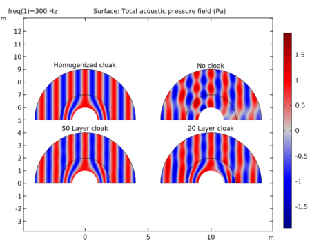
In the window for , type Total Acoustic Pressure (acpr) in the text field.

Locate the section. Clear the check box.

Line 1

Right-click and choose .

In the window for , locate the section.

In the text field, type 0.

Click to expand the section. From the list, choose .

Locate the section. From the list, choose .

From the list, choose .

Selection 1

Right-click and choose .

Select Boundaries 1, 2, 105–108, 151–156, and 208–211 only.

In the toolbar, click .

Annotation 1

In the window, right-click and choose .

In the window for , locate the section.

In the text field, type Homogenized cloak.

Locate the section. In the text field, type x1.

In the text field, type y1+4.3.

Locate the section. Clear the check box.

From the list, choose .

Annotation 2

Right-click and choose .

In the window for , locate the section.

In the text field, type No cloak.

Locate the section. In the text field, type x2.

In the text field, type y2+4.3.

Locate the section. Clear the check box.

From the list, choose .

Annotation 3

Right-click and choose .

In the window for , locate the section.

In the text field, type 50 Layer cloak.

Locate the section. In the text field, type x3.

In the text field, type y3+4.3.

Locate the section. Clear the check box.

From the list, choose .

Annotation 4

Right-click and choose .

In the window for , locate the section.

In the text field, type 20 Layer cloak.

Locate the section. In the text field, type x4.

In the text field, type y4+4.3.

Locate the section. Clear the check box.

From the list, choose .

Total Acoustic Pressure (acpr)

In the window, click .

In the toolbar, click .

The plot should look like that in Figure 2.

Sound Pressure Level (acpr)

In the window, right-click and choose .

Remove the default Sound Pressure Level plot and duplicate the Total Acoustic Pressure plot created previously. Doing this, you make sure that the annotations will be carried over to the new plots.

Total Acoustic Pressure (acpr) 1

In the window, right-click and choose .

In the window for , type Total Sound Pressure Level (acpr) in the text field.

Surface 1

In the window, expand the node, then click .

In the window for , locate the section.

In the text field, type acpr.Lp.

Locate the section. From the list, choose .

Clear the check box.

In the toolbar, click .

The plot should look like that in Figure 3.

Total Sound Pressure Level (acpr) 1

In the window, right-click and choose .

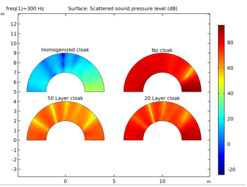
In the window for , type Scattered Sound Pressure Level (acpr) in the text field.

Surface 1

In the window, expand the node, then click .

In the window for , locate the section.

In the text field, type acpr.Lp_s.

Selection 1

Right-click and choose .

Select Domains 1, 2, 54, and 55 only.

In the toolbar, click .

The plot should look like that in Figure 4.

1D Plot Group 4

In the toolbar, click and choose .

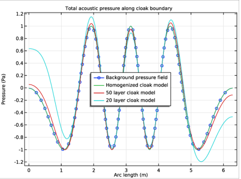
In the window for , type Total Acoustic Pressure Along Cloak Boundary in the text field.

Click to expand the section. From the list, choose .

In the text area, type Total acoustic pressure along cloak boundary.

Locate the section. Select the check box.

In the associated text field, type Pressure (Pa).

Locate the section. From the list, choose .

Line Graph 1

Right-click and choose .

Select Boundary 156 only.

In the window for , locate the section.

In the text field, type acpr.p_b.

Click to expand the section. From the list, choose .

Click to expand the section. Select the check box.

From the list, choose .

Select Boundary 155 only.


Legends
Background pressure field

Click to expand the section. Find the subsection. From the list, choose .

In the text field, type 100.

In the toolbar, click .

Line Graph 2

Right-click and choose .

In the window for , locate the section.

In the text field, type acpr.p_t.

Locate the section. Find the subsection. From the list, choose .

Locate the section. In the table, enter the following settings:


Legends
Homogenized cloak model

Line Graph 3

Right-click and choose .

In the window for , locate the section.

Click .

Locate the section. In the table, enter the following settings:


Legends
50 layer cloak model

Line Graph 4

Right-click and choose .

In the window for , locate the section.

Click .

Select Boundary 210 only.

Locate the section. In the table, enter the following settings:


Legends
20 layer cloak model

In the toolbar, click .

The plot should look like that in Figure 5.

1D Plot Group 5

In the toolbar, click and choose .

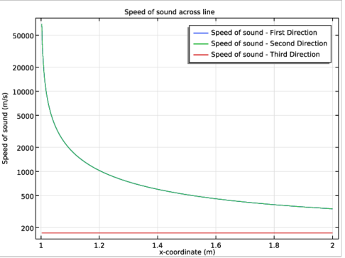
In the window for , type Speed of Sound in the Homogenized Material in the text field.

Locate the section. Select the check box.

In the associated text field, type Speed of sound (m/s).

Locate the section. From the list, choose .

In the text area, type Speed of sound across line.

Line Graph 1

Right-click and choose .

Select Boundary 55 only.

In the window for , locate the section.

In the text field, type sqrt(matdiag1.e1)[m/s].

Select the check box.

In the associated text field, type Speed of sound - First direction.

Locate the section. From the list, choose .

In the text field, type x.

Locate the section. Select the check box.

From the list, choose .

The plot should look like that in Figure 6.


Legends
Speed of sound - First Direction

Line Graph 2

Right-click and choose .

In the window for , locate the section.

In the text field, type sqrt(matdiag1.e2)[m/s].

In the text field, type Speed of sound - Second direction.

Locate the section. In the table, enter the following settings:


Legends
Speed of sound - Second Direction

Line Graph 3

Right-click and choose .

In the window for , locate the section.

In the text field, type sqrt(matdiag1.e3)[m/s].

In the text field, type Speed of sound - Third direction.

Locate the section. In the table, enter the following settings:


Legends
Speed of sound - Third Direction

Click the button in the toolbar.

In the toolbar, click .

Appendix: Geometry Sequence Instructions

Add Component

In the toolbar, click and choose .

Global Definitions

Parameters 1

In the window, under click .

In the window for , locate the section.

Click .

Browse to the model’s Application Libraries folder and double-click the file acoustic_cloaking_geom_sequence_parameters.txt.

Geometry 1

Circle 1 (c1)

In the toolbar, click .

In the window for , locate the section.

In the text field, type 4.

In the text field, type 180.

Locate the section. In the text field, type x1.

In the text field, type y1.

Click to expand the section. In the table, enter the following settings:


Layer name	Thickness (m)
Layer 1	R2
Layer 2	R1

Circle 2 (c2)

In the toolbar, click .

In the window for , locate the section.

In the text field, type 2*R2.

In the text field, type 180.

Locate the section. In the text field, type x2.

In the text field, type y2.

Locate the section. In the table, enter the following settings:


Layer name	Thickness (m)
Layer 1	R2
Layer 2	R1

Circle 3 (c3)

In the toolbar, click .

In the window for , locate the section.

In the text field, type 2*R2.

In the text field, type 180.

Locate the section. In the text field, type x3.

In the text field, type y3.

Locate the section. In the table, enter the following settings:


Layer name	Thickness (m)
Layer 1	R2
Layer 2	(R2-R1)/50
Layer 3	(R2-R1)/50
Layer 4	(R2-R1)/50
Layer 5	(R2-R1)/50
Layer 6	(R2-R1)/50
Layer 7	(R2-R1)/50
Layer 8	(R2-R1)/50
Layer 9	(R2-R1)/50
Layer 10	(R2-R1)/50
Layer 11	(R2-R1)/50
Layer 12	(R2-R1)/50
Layer 13	(R2-R1)/50
Layer 14	(R2-R1)/50
Layer 15	(R2-R1)/50
Layer 16	(R2-R1)/50
Layer 17	(R2-R1)/50
Layer 18	(R2-R1)/50
Layer 19	(R2-R1)/50
Layer 20	(R2-R1)/50
Layer 21	(R2-R1)/50
Layer 22	(R2-R1)/50
Layer 23	(R2-R1)/50
Layer 24	(R2-R1)/50
Layer 25	(R2-R1)/50
Layer 26	(R2-R1)/50
Layer 27	(R2-R1)/50
Layer 28	(R2-R1)/50
Layer 29	(R2-R1)/50
Layer 30	(R2-R1)/50
Layer 31	(R2-R1)/50
Layer 32	(R2-R1)/50
Layer 33	(R2-R1)/50
Layer 34	(R2-R1)/50
Layer 35	(R2-R1)/50
Layer 36	(R2-R1)/50
Layer 37	(R2-R1)/50
Layer 38	(R2-R1)/50
Layer 39	(R2-R1)/50
Layer 40	(R2-R1)/50
Layer 41	(R2-R1)/50
Layer 42	(R2-R1)/50
Layer 43	(R2-R1)/50
Layer 44	(R2-R1)/50
Layer 45	(R2-R1)/50
Layer 46	(R2-R1)/50
Layer 47	(R2-R1)/50
Layer 48	(R2-R1)/50
Layer 49	(R2-R1)/50
Layer 50	(R2-R1)/50
Layer 51	(R2-R1)/50

Circle 4 (c4)

In the toolbar, click .

In the window for , locate the section.

In the text field, type 2*R2.

In the text field, type 180.

Locate the section. In the text field, type x4.

In the text field, type y4.

Locate the section. In the table, enter the following settings:


Layer name	Thickness (m)
Layer 1	R2
Layer 2	(R2-R1)/20
Layer 3	(R2-R1)/20
Layer 4	(R2-R1)/20
Layer 5	(R2-R1)/20
Layer 6	(R2-R1)/20
Layer 7	(R2-R1)/20
Layer 8	(R2-R1)/20
Layer 9	(R2-R1)/20
Layer 10	(R2-R1)/20
Layer 11	(R2-R1)/20
Layer 12	(R2-R1)/20
Layer 13	(R2-R1)/20
Layer 14	(R2-R1)/20
Layer 15	(R2-R1)/20
Layer 16	(R2-R1)/20
Layer 17	(R2-R1)/20
Layer 18	(R2-R1)/20
Layer 19	(R2-R1)/20
Layer 20	(R2-R1)/20
Layer 21	(R2-R1)/20

Click .

Click the button in the toolbar.

Delete Entities 1 (del1)

In the window, right-click and choose .

In the window for , locate the section.

From the list, choose .

On the object , select Domain 3 only.

On the object , select Domain 52 only.

On the object , select Domain 22 only.

Click .

The geometry should look like this.

Now that the geometry has been generated, you can proceed to simplify some of its features.

Ignore Edges 1 (ige1)

In the toolbar, click and choose .

In the window for , locate the section.

Clear the check box.

Click .

In the dialog box, type 54-106 183-205 in the text field.

In the window for , click .

Ignore Vertices 1 (igv1)

In the toolbar, click and choose .

In the window for , locate the section.

Click .

In the dialog box, type 56-110 191-215 in the text field.

With this clean geometry, you can proceed to generate a few selections that will be used in the model.

In the window for , click .

Geometry 1

Explicit Selection 1 (sel1)

In the toolbar, click and choose .

In the window for , type Selection: Material 1 in the text field.

Locate the section. Click .

In the dialog box, type igv1: 5, 7, 9, 11, 13, 15, 17, 19, 21, 23, 25, 27, 29, 31, 33, 35, 37, 39, 41, 43, 45, 47, 49, 51, 53, 58, 60, 62, 64, 66, 68, 70, 72, 74, 76 in the text field.

Explicit Selection 2 (sel2)

In the toolbar, click and choose .

In the window for , type Selection: Material 2 in the text field.

Locate the section. Click .

In the dialog box, type igv1: 3, 6, 8, 10, 12, 14, 16, 18, 20, 22, 24, 26, 28, 30, 32, 34, 36, 38, 40, 42, 44, 46, 48, 50, 52, 56, 59, 61, 63, 65, 67, 69, 71, 73, 75 in the text field.