|
|
|

|
1
|
|
2
|
In the Select Physics tree, select AC/DC>Electromagnetic Fields>Vector Formulations>Magnetic Field Formulation (mfh).
|
|
3
|
Click Add.
|
|
4
|
Click Study.
|
|
5
|
|
6
|
Click Done.
|
|
1
|
|
1
|
|
2
|
|
3
|
|
4
|
|
1
|
|
2
|
|
3
|
|
4
|
Browse to the model’s Application Libraries folder and double-click the file superconducting_wire_parameters.txt.
|
|
1
|
|
2
|
|
1
|
|
2
|
In the Show More Options dialog box, in the tree, select the check box for the node Physics>Advanced Physics Options.
|
|
3
|
Click OK.
|
|
4
|
|
5
|
In the Settings window for Magnetic Field Formulation, click to expand the Divergence Constraint section.
|
|
6
|
|
1
|
In the Model Builder window, under Component 1 (comp1)>Magnetic Field Formulation (mfh) click Faraday’s Law 1.
|
|
2
|
|
3
|
|
1
|
|
3
|
|
4
|
|
1
|
|
3
|
|
4
|
|
5
|
|
1
|
In the Model Builder window, under Component 1 (comp1) right-click Materials and choose Blank Material.
|
|
2
|
|
3
|
|
4
|
Click OK.
|
|
5
|
|
Ω·m
|
||||
|
1
|
|
2
|
|
3
|
|
4
|
Click OK.
|
|
6
|
|
8
|
Click to expand the Material Properties section. In the Material properties tree, select Electromagnetic Models>E-J Characteristic.
|
|
9
|
|
10
|
|
1
|
|
2
|
|
3
|
|
5
|
|
6
|
|
1
|
|
2
|
|
3
|
|
4
|
|
1
|
|
2
|
|
3
|
Click Range.
|
|
4
|
|
5
|
|
6
|
Click Replace.
|
|
1
|
|
2
|
|
3
|
|
4
|
|
6
|
|
7
|
|
8
|
In the Model Builder window, expand the Study 1>Solver Configurations>Solution 1 (sol1)>Time-Dependent Solver 1 node, then click Fully Coupled 1.
|
|
9
|
|
10
|
|
11
|
|
1
|
|
2
|
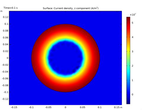
In the Settings window for Surface, click Replace Expression in the upper-right corner of the Expression section. From the menu, choose Component 1>Magnetic Field Formulation>Currents and charge>Current density - A/m²>mfh.Jz - Current density, z component.
|
|
3
|
|
4
|
Click the Zoom In button on the Graphics toolbar two or three times to get a closer view of the wire.
|
|
1
|
|
2
|
|
3
|
|
4
|