Magnetic Signature of a Submarine

A vessel traveling on the surface or under water gives rise to detectable local disturbances in the Earth’s magnetic field. These disturbances can be used to trigger weapon systems. The magnetic signature of a ship can be reduced by generating a counteracting magnetic field of suitable strength and direction based on prior knowledge of the magnetic properties of the vessel. An important step in the design of a naval ship is therefore to predict its magnetic signature. Another application where magnetic signatures are of great importance is in urban traffic control: magnetic sensors, buried in our streets, are used to sense vehicles and control traffic lights.

Ships and cars are both to a large extent made of sheet metal. This makes them hard to simulate using standard finite element analysis because volume meshes of thin extended structures are difficult to generate and tend to become very large. This application demonstrates a powerful technique that circumvents the problem by modeling the sheet metal as 2D faces embedded in a 3D geometry. Thus it is only necessary to create comparatively inexpensive 2D face meshes in addition to the 3D volume mesh used for the surrounding medium. A tangential projection of the 3D equation is then solved on the 2D face mesh.

Figure 1: Submarine HMAS Collins. Image courtesy of Kockums AB.

This application also demonstrates the use of the reduced field formulation available in the AC/DC Module. This feature provides a convenient way to obtain the magnetic signature of the submarine by allowing the user to define the background field as a predefined quantity and solving only for the perturbations in this field.

Model Definition

In magnetostatic problems, where no currents are present, the problem can be solved using a scalar magnetic potential. This application demonstrates a special technique for modeling thin sheets of high permeability materials, and also shows the use of the reduced field formulation in the AC/DC Module for conveniently modeling perturbations in a known background field.

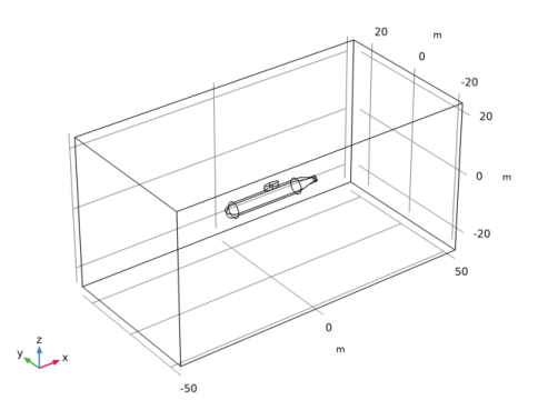
The model geometry is shown in Figure 2 and consists of face objects representing the submarine. A 3D box representing the surrounding water encloses the vessel.

Figure 2: The model geometry.

Domain Equations

In a current-free region, where

it is possible to define the scalar magnetic potential, Vm, from the relation

This is analogous to the definition of the electric potential for static electric fields. Using the constitutive relation between the magnetic flux density and magnetic field

together with the equation

you can derive an equation for Vm,

In this model you use the reduced field formulation, which means that you only solve for the potential Vm corresponding to the perturbation (reduced) field, so the equation you solve reads

where Bext is a known background field, in this case the Earth’s magnetic field of 0.5 G.

Boundary Conditions

The exterior boundaries of the box are insulating for the reduced magnetic field:

On the face objects representing the hull of the submarine, you apply a 2D tangential projection of the 3D domain equation where the thickness and permeability of the hull are introduced as parameters. This is readily available in the used formulation as a shielding boundary condition, which is useful for modeling of highly permeable thin sheets. Corresponding boundary conditions are available in the Electric Currents and Electrostatics interfaces for modeling of thin sheets with high conductance and high permittivity respectively.

Results and Discussion

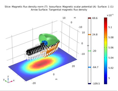
Figure 3 shows the total magnetic flux density in a horizontal slice plot 12.5 m below the keel of the submarine. A distinct field perturbation due to the presence of the vessel can be seen. The magnitude and direction of the tangential magnetic field in the hull of the vessel is shown using arrows. The reduced field is visualized as isolevels of the reduced magnetic potential. This gives a good picture of the perturbation caused by the presence of the submarine in the background field.