PDF

Computing the Resistance of a Wire
Introduction
Applying a voltage difference to a conductor creates a current flow and the intensity of the current is usually a function of the applied voltage difference. In the simplest (linear) case, the current flow and the voltage difference are proportional; the proportionality constant is the resistance of the device. This model demonstrates how to compute the resistance of a short section of copper wire. The convergence of the solution with respect to the mesh size is also studied.
Figure 1: A short section of copper wire. The objective is to compute the equivalent resistance of this wire.
Model Definition
A 10 mm long section of copper wire of 1 mm radius, as shown in Figure 1, is studied. A constant current of 1 A is passed through the wire and the voltage drop is measured, from which the resistance of the wire is computed.
The boundary conditions used are meant to represent a connection to a DC source of current. One end of the wire is grounded, representing a current sink, and the other end is connected to a constant current source of 1 A, using the Terminal boundary condition.
Three different meshes are studied, to demonstrate that the results are converged with respect to mesh refinement — any further refinement of the mesh would only marginally improve the precision of the results. A Free Tetrahedral mesh is used, with varying default element sizes. The results are compared, and mesh convergence is shown.
Results and Discussion
The voltage distribution is plotted in Figure 2. A linear drop in the voltage along the length of the wire can be observed. The resistance of this 10 mm long wire is computed to be 0.212 mΩ., a value that agrees within 1% for all meshes.
Figure 2: The voltage decreases linearly along the length of the wire.
Application Library path: ACDC_Module/Resistive_Devices/simple_resistor
Modeling Instructions
From the File menu, choose New.
New
In the New window, click Model Wizard.
Model Wizard
1
In the Model Wizard window, click 3D.
2
In the Select Physics tree, select AC/DC>Electric Fields and Currents>Electric Currents (ec).
3
Click Add.
4
Click Study.
5
In the Select Study tree, select General Studies>Stationary.
6
Click Done.
Geometry 1
Begin by creating a cylinder for the copper wire.
Cylinder 1 (cyl1)
1
In the Geometry toolbar, click Cylinder.
2
In the Settings window for Cylinder, locate the Size and Shape section.
3
In the Radius text field, type 0.5[mm].
4
In the Height text field, type 10[mm].
5
Click Build All Objects.
6
Click the Wireframe Rendering button in the Graphics toolbar.
Electric Currents (ec)
Set up the Electric Current physics. Specify the ground and terminal boundaries.
Ground 1
1
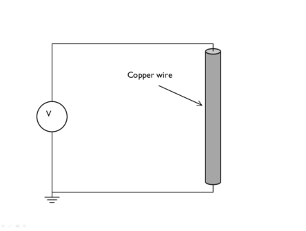
In the Model Builder window, under Component 1 (comp1) right-click Electric Currents (ec) and choose Ground.
2
Terminal 1
1
In the Physics toolbar, click Boundaries and choose Terminal.
2
3
In the Settings window for Terminal, locate the Terminal section.
4
In the I0 text field, type 1.
Materials
Then, assign material properties. Use copper for all domains.
Add Material
1
In the Home toolbar, click Add Material to open the Add Material window.
2
Go to the Add Material window.
3
In the tree, select Built-in>Copper.
4
Click Add to Component in the window toolbar.
5
In the Home toolbar, click Add Material to close the Add Material window.
Mesh 1
Free Tetrahedral 1
In the Model Builder window, under Component 1 (comp1) right-click Mesh 1 and choose Free Tetrahedral.
Size
1
In the Settings window for Size, locate the Element Size section.
2
From the Predefined list, choose Extra coarse.
3
Click Build All.
Study 1
In the Home toolbar, click Compute.
Results
Electric Potential (ec)
The default plot shows the electric potential in the copper wire. See Figure 2.
Derived Values
Evaluate the resistance of the wire with the extra coarse mesh size.
Global Evaluation 1
1
In the Results toolbar, click Global Evaluation.
2
In the Settings window for Global Evaluation, click Replace Expression in the upper-right corner of the Expressions section. From the menu, choose Component 1>Electric Currents>Terminals>ec.R11 - Resistance - Ω.
3
Locate the Expressions section. In the table, enter the following settings:
mΩ
4
Click Evaluate.
Mesh 1
Size
1
In the Model Builder window, under Component 1 (comp1)>Mesh 1 click Size.
2
In the Settings window for Size, locate the Element Size section.
3
From the Predefined list, choose Normal.
4
Click Build All.
Study 1
In the Home toolbar, click Compute.
Results
Global Evaluation 1
Evaluate the resistance of the wire with the normal mesh size.
1
In the Model Builder window, under Results>Derived Values click Global Evaluation 1.
2
Click Evaluate.
Mesh 1
Size
1
In the Model Builder window, under Component 1 (comp1)>Mesh 1 click Size.
2
In the Settings window for Size, locate the Element Size section.
3
From the Predefined list, choose Extra fine.
4
Click Build All.
Study 1
In the Home toolbar, click Compute.
Results
Global Evaluation 1
Finish the result analysis by evaluating the resistance of the wire with the extra fine mesh size.
1
In the Model Builder window, under Results>Derived Values click Global Evaluation 1.
2
Click Evaluate.
Table
1
Go to the Table window.
The evaluated wire resistance for the three different meshes should agree within 1%.