PDF

Quadrupole Mass Spectrometer
Introduction
The principal component of a quadrupole mass spectrometer is the mass filter which is used to filter ions with different charge-to-mass ratios. The quadrupole mass filter has been studied over many years (Ref. 1) and the physics and optimal design are well understood. In a real quadrupole mass spectrometer, fringe fields exist at both the entrance and exit of the mass filter. These fringe fields can play an important role in determining the transmission probability of a specific ion through the mass filter. This model computes the ion trajectories in a quadrupole mass spectrometer, including the effects of fringe fields.
Note: This application requires the Particle Tracing Module.
Model Definition
For the DC field, Poisson’s equation is solved for the electric potential, U:
(1)
where ε0 is the permittivity of free space (SI unit: F/m) and εr is the relative permittivity (taken as 1 in this model). The zero on the right-hand side of Equation 1 indicates that the space charge density inside the quadrupole is negligible (Ref. 1). On the north and south rods, a positive potential of magnitude Udc is applied:
and on the east and west rods, a negative potential is applied:
A small DC bias is applied on the ion aperture to help accelerate the ions into the mass filter:
where Ubias is taken to be 3 V.
For the AC fields, the conservation of electric currents is used to compute the AC potential, V:
where σ is the electrical conductivity in the mass filter (taken as zero here) and ω is the angular frequency (SI unit: Hz).
On the north and south rods, a positive potential of magnitude Vac is applied:
and on the east and west rods, a negative potential is applied:
A small AC bias is applied on the ion aperture to help accelerate the ions into the mass filter:
where Vbias is taken to be 3 V.
To construct the total electric field which the particles experience once they enter the modeling domain, the model uses superposition of the AC and DC fields. This is a valid assumption in this case because the equations solved for the AC and DC fields are linear.
Newton’s second law governs the particle motion:
Here m is the particle mass (SI unit: kg), v is the particle velocity (SI unit: m/s), Z is the dimensionless charge number, e is the elementary charge (SI unit: s A), and E is the electric field (SI unit: V/m). The electric field contains two contributions, a stationary electric field and one which is changing over time:
where
and
where the tilde denotes that the AC electric potential is complex valued. The particle position, q, is simply computed from the definition of the velocity:
The particles are released from the ion aperture with a thermal velocity the equivalent of 2 electron volts, Ref. 1. The velocity only has an x-component:
where A is 2 eV. Particles are not only released at the simulation start time, they must be released at uniformly spaced times over the first RF cycle of the AC field. Particles are released at 11 times beginning at 0 s and ending at 0.25 μs. Because the frequency of the AC field is 4 MHz, this corresponds to one full RF cycle.
Results and Discussion
The particle trajectories are plotted in Figure 1. It is obvious from the plot that the ion transmission probability is very high, 100% actually. This is because a very stable operating point on the a-q curve has been chosen. The ions remain in the quadrupole mass filter for around 140 RF cycles.
Due to the presence of the biased plate surrounding the ion aperture, the ions gain energy as they move through the quadrupole. This can be seen in Figure 2; the ions have a mean energy of 5 eV over a range of around 3 eV. The spread in energy can be attributed to the fact that there is a small DC and AC bias. The AC bias can be positive or negative which accelerates or decelerates the ions depending on the phase of the RF cycle when they are released.
Figure 1: Plot of the particle trajectories inside the quadrupole. The color represents the particle velocity (m/s).
Figure 2: Plot of the energy distribution of the ions at the collector.
Notes About the COMSOL Implementation
The model is solved in two stages. First, the DC and AC fields are computed. Then the particle trajectories are computed and their motion is driven by the AC and DC electric fields.
Reference
1. J.R. Gibson, S. Taylor, and J.H. Leck, “Detailed simulation of mass spectra for quadrupole mass spectrometer systems,” J. Vac. Sci. Technol. A, vol. 18, no. 1, p. 237, 2000.
Application Library path: ACDC_Module/Particle_Tracing/quadrupole_mass_spectrometer
Modeling Instructions
From the File menu, choose New.
New
In the New window, click Model Wizard.
Model Wizard
1
In the Model Wizard window, click 3D.
2
In the Select Physics tree, select AC/DC>Electric Fields and Currents>Electrostatics (es).
3
Click Add.
4
In the Select Physics tree, select AC/DC>Electric Fields and Currents>Electric Currents (ec).
5
Click Add.
6
In the Select Physics tree, select AC/DC>Particle Tracing>Charged Particle Tracing (cpt).
7
Click Add.
8
Click Done.
Global Definitions
Add some parameters for the quadrupole geometry and physics settings. To save time, the parameters can be loaded from a file.
Parameters 1
1
In the Model Builder window, under Global Definitions click Parameters 1.
2
In the Settings window for Parameters, locate the Parameters section.
3
Click Load from File.
4
Geometry 1
Work Plane 1 (wp1)
1
In the Geometry toolbar, click Work Plane.
2
In the Settings window for Work Plane, locate the Plane Definition section.
3
From the Plane list, choose yz-plane.
4
Click Show Work Plane.
Work Plane 1 (wp1)>Circle 1 (c1)
1
In the Work Plane toolbar, click Circle.
2
In the Settings window for Circle, locate the Size and Shape section.
3
In the Radius text field, type re.
4
Locate the Position section. In the xw text field, type -(re+r0).
Work Plane 1 (wp1)>Circle 2 (c2)
1
In the Work Plane toolbar, click Circle.
2
In the Settings window for Circle, locate the Size and Shape section.
3
In the Radius text field, type re.
4
Locate the Position section. In the xw text field, type re+r0.
Work Plane 1 (wp1)>Circle 3 (c3)
1
In the Work Plane toolbar, click Circle.
2
In the Settings window for Circle, locate the Size and Shape section.
3
In the Radius text field, type re.
4
Locate the Position section. In the yw text field, type -(re+r0).
Work Plane 1 (wp1)>Circle 4 (c4)
1
In the Work Plane toolbar, click Circle.
2
In the Settings window for Circle, locate the Size and Shape section.
3
In the Radius text field, type re.
4
Locate the Position section. In the yw text field, type re+r0.
5
In the Work Plane toolbar, click Build All.
6
Click the Zoom Extents button in the Graphics toolbar.
Work Plane 1 (wp1)
In the Model Builder window, click Work Plane 1 (wp1).
Extrude 1 (ext1)
1
In the Geometry toolbar, click Extrude.
2
In the Settings window for Extrude, locate the Distances section.
3
4
Click Build All Objects.
5
Click the Zoom Extents button in the Graphics toolbar.
Work Plane 2 (wp2)
1
In the Geometry toolbar, click Work Plane.
2
In the Settings window for Work Plane, locate the Plane Definition section.
3
From the Plane list, choose yz-plane.
4
In the x-coordinate text field, type -fd.
5
Click Show Work Plane.
Work Plane 2 (wp2)>Circle 1 (c1)
1
In the Work Plane toolbar, click Circle.
2
In the Settings window for Circle, locate the Size and Shape section.
3
In the Radius text field, type rcase.
Work Plane 2 (wp2)>Circle 2 (c2)
1
In the Work Plane toolbar, click Circle.
2
In the Settings window for Circle, locate the Size and Shape section.
3
In the Radius text field, type rsrc.
Work Plane 2 (wp2)>Circle 3 (c3)
1
In the Work Plane toolbar, click Circle.
2
In the Settings window for Circle, locate the Size and Shape section.
3
In the Radius text field, type 2*rsrc.
4
In the Work Plane toolbar, click Build All.
5
Click the Zoom Extents button in the Graphics toolbar.
Work Plane 2 (wp2)
In the Model Builder window, click Work Plane 2 (wp2).
Extrude 2 (ext2)
1
In the Geometry toolbar, click Extrude.
2
In the Settings window for Extrude, locate the Distances section.
3
4
Click Build All Objects.
Difference 1 (dif1)
1
In the Geometry toolbar, click Booleans and Partitions and choose Difference.
2
3
In the Settings window for Difference, locate the Difference section.
4
Find the Objects to subtract subsection. Select the Activate selection toggle button.
5
6
Click Build All Objects.
7
Click the Zoom Extents button in the Graphics toolbar.
Now define some selections for the positively and negatively charged rods.
Definitions
Explicit 1
1
In the Definitions toolbar, click Explicit.
2
In the Settings window for Explicit, type Positive in the Label text field.
3
Click the Wireframe Rendering button in the Graphics toolbar.
4
Locate the Input Entities section. From the Geometric entity level list, choose Boundary.
5
Explicit 2
1
In the Definitions toolbar, click Explicit.
2
In the Settings window for Explicit, type Negative in the Label text field.
3
Locate the Input Entities section. From the Geometric entity level list, choose Boundary.
4
Electrostatics (es)
Define the boundary conditions for the electrostatics problem.
Electric Potential 1
1
In the Model Builder window, under Component 1 (comp1) right-click Electrostatics (es) and choose Electric Potential.
2
In the Settings window for Electric Potential, locate the Boundary Selection section.
3
From the Selection list, choose Positive.
4
Locate the Electric Potential section. In the V0 text field, type Udc.
Electric Potential 2
1
In the Physics toolbar, click Boundaries and choose Electric Potential.
2
In the Settings window for Electric Potential, locate the Boundary Selection section.
3
From the Selection list, choose Negative.
4
Locate the Electric Potential section. In the V0 text field, type -Udc.
Electric Potential 3
1
In the Physics toolbar, click Boundaries and choose Electric Potential.
2
3
In the Settings window for Electric Potential, locate the Electric Potential section.
4
In the V0 text field, type 3.
Electric Currents (ec)
Now define the boundary conditions for the AC part of the problem.
1
In the Model Builder window, under Component 1 (comp1) click Electric Currents (ec).
Electric Potential 1
1
In the Physics toolbar, click Boundaries and choose Electric Potential.
2
In the Settings window for Electric Potential, locate the Boundary Selection section.
3
From the Selection list, choose Positive.
4
Locate the Electric Potential section. In the V0 text field, type Vac.
Electric Potential 2
1
In the Physics toolbar, click Boundaries and choose Electric Potential.
2
In the Settings window for Electric Potential, locate the Boundary Selection section.
3
From the Selection list, choose Negative.
4
Locate the Electric Potential section. In the V0 text field, type -Vac.
Electric Potential 3
1
In the Physics toolbar, click Boundaries and choose Electric Potential.
2
3
In the Settings window for Electric Potential, locate the Electric Potential section.
4
In the V0 text field, type 3.
Specify the mass and charge number of the ions.
Charged Particle Tracing (cpt)
Particle Properties 1
1
In the Model Builder window, under Component 1 (comp1)>Charged Particle Tracing (cpt) click Particle Properties 1.
2
In the Settings window for Particle Properties, locate the Particle Mass section.
3
In the mp text field, type mi.
4
Locate the Charge Number section. In the Z text field, type 1.
The particles are released from a projected plane grid on the Inlet boundary. There are 100 particles per release and 11 releases in total. The particles all move in the x-direction with initial energy 2 eV.
Inlet 1
1
In the Physics toolbar, click Boundaries and choose Inlet.
2
3
In the Settings window for Inlet, locate the Initial Position section.
4
From the Initial position list, choose Projected plane grid.
5
In the N text field, type 100.
6
Locate the Release Times section. Click Range.
7
In the Range dialog box, choose Number of values from the Entry method list.
8
In the Start text field, type 0.
9
In the Stop text field, type 1/4E6.
10
In the Number of values text field, type 11.
11
Click Replace.
12
In the Settings window for Inlet, locate the Initial Velocity section.
13
Specify the v0 vector as
Add an Electric Force feature for the DC field.
Electric Force 1
1
In the Physics toolbar, click Domains and choose Electric Force.
2
In the Settings window for Electric Force, locate the Electric Force section.
3
From the E list, choose Electric field (es/ccn1).
4
Locate the Domain Selection section. From the Selection list, choose All domains.
Add another Electric Force feature for the AC field.
Electric Force 2
1
In the Physics toolbar, click Domains and choose Electric Force.
2
In the Settings window for Electric Force, locate the Electric Force section.
3
From the E list, choose Electric field (ec/cucn1).
4
Locate the Advanced Settings section. From the Time dependence of field list, choose Time harmonic.
5
Locate the Domain Selection section. From the Selection list, choose All domains.
Materials
Material 1 (mat1)
1
In the Model Builder window, under Component 1 (comp1) right-click Materials and choose Blank Material.
2
In the Settings window for Material, locate the Material Contents section.
3
Since the aspect ratio of the quadrupole is very high, it is more efficient to use a swept mesh. This is allowed in this case because the field does not change in the x-direction once the particles have passed through the fringing fields.
Mesh 1
Free Triangular 1
1
In the Model Builder window, under Component 1 (comp1) right-click Mesh 1 and choose More Operations>Free Triangular.
2
Size 1
1
Right-click Free Triangular 1 and choose Size.
2
In the Settings window for Size, locate the Element Size section.
3
From the Predefined list, choose Extra fine.
4
Click to expand the Element Size Parameters section. Locate the Element Size section. Click the Custom button.
5
Locate the Element Size Parameters section. Select the Maximum element size check box.
6
Select the Minimum element size check box.
7
Select the Curvature factor check box.
8
9
Click Build All.
Swept 1
1
In the Model Builder window, right-click Mesh 1 and choose Swept.
2
In the Settings window for Swept, locate the Domain Selection section.
3
From the Geometric entity level list, choose Domain.
4
Distribution 1
1
Right-click Swept 1 and choose Distribution.
2
In the Settings window for Distribution, locate the Distribution section.
3
From the Distribution type list, choose Predefined.
4
In the Number of elements text field, type 35.
5
In the Element ratio text field, type 15.
6
Click Build All.
7
Click the Go to Default View button in the Graphics toolbar.
Swept 2
1
In the Model Builder window, right-click Mesh 1 and choose Swept.
2
In the Settings window for Swept, locate the Domain Selection section.
3
From the Geometric entity level list, choose Domain.
4
Distribution 1
1
Right-click Swept 2 and choose Distribution.
2
Click Build All.
Add a Stationary study to compute the electrostatic field.
Add Study
1
In the Home toolbar, click Add Study to open the Add Study window.
2
Go to the Add Study window.
3
Find the Studies subsection. In the Select Study tree, select Preset Studies for Some Physics Interfaces>Stationary.
4
Click Add Study in the window toolbar.
5
In the Home toolbar, click Add Study to close the Add Study window.
Study 1
Step 1: Stationary
1
In the Settings window for Stationary, locate the Physics and Variables Selection section.
2
In the table, clear the Solve for check box for Electric Currents and Charged Particle Tracing.
3
In the Model Builder window, right-click Study 1 and choose Rename.
4
In the Rename Study dialog box, type Electrostatic Study in the New label text field.
5
Add a Frequency Domain study to compute the AC field.
Add Study
1
In the Home toolbar, click Add Study to open the Add Study window.
2
Go to the Add Study window.
3
Find the Studies subsection. In the Select Study tree, select Preset Studies for Some Physics Interfaces>Frequency Domain.
4
Click Add Study in the window toolbar.
5
In the Home toolbar, click Add Study to close the Add Study window.
Study 2
Step 1: Frequency Domain
1
In the Settings window for Frequency Domain, locate the Study Settings section.
2
In the Frequencies text field, type 4[MHz].
3
Locate the Physics and Variables Selection section. In the table, clear the Solve for check box for Electrostatics and Charged Particle Tracing.
4
Click to expand the Values of Dependent Variables section. Find the Values of variables not solved for subsection. From the Settings list, choose User controlled.
5
From the Method list, choose Solution.
6
From the Study list, choose Electrostatic Study, Stationary.
7
In the Model Builder window, right-click Study 2 and choose Rename.
8
In the Rename Study dialog box, type Electric currents Study in the New label text field.
9
Add a Time Dependent study to compute the particle trajectories.
Add Study
1
In the Home toolbar, click Add Study to open the Add Study window.
2
Go to the Add Study window.
3
Find the Studies subsection. In the Select Study tree, select General Studies>Time Dependent.
4
Click Add Study in the window toolbar.
5
In the Home toolbar, click Add Study to close the Add Study window.
Study 3
Step 1: Time Dependent
1
In the Settings window for Time Dependent, locate the Physics and Variables Selection section.
2
In the table, clear the Solve for check box for Electrostatics and Electric Currents.
3
Click to expand the Values of Dependent Variables section. Find the Values of variables not solved for subsection. From the Settings list, choose User controlled.
4
From the Method list, choose Solution.
5
From the Study list, choose Electric currents Study, Frequency Domain.
6
Locate the Study Settings section. In the Times text field, type range(0,1/4e6,140/4e6).
7
Click Range.
8
In the Range dialog box, click Replace.
9
In the Model Builder window, right-click Study 3 and choose Rename.
10
In the Rename Study dialog box, type Particle tracing Study in the New label text field.
11
Electrostatic Study
Compute the DC field.
1
In the Home toolbar, click Compute.
Electric currents Study
Compute the AC field.
1
Click Compute.
Particle tracing Study
Now, compute the particle trajectories.
1
Click Compute.
Results
Particle Trajectories (cpt)
1
In the Settings window for 3D Plot Group, locate the Color Legend section.
2
From the Position list, choose Bottom.
Particle Trajectories 1
1
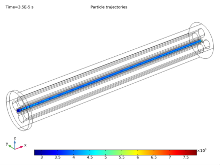
In the Model Builder window, expand the Particle Trajectories (cpt) node, then click Particle Trajectories 1.
2
In the Settings window for Particle Trajectories, locate the Coloring and Style section.
3
Find the Line style subsection. From the Type list, choose Line.
4
Find the Point style subsection. From the Type list, choose None.
5
Find the Line style subsection. From the Interpolation list, choose Uniform.
6
In the Number of interpolated times text field, type 1000.
Definitions
View 1
1
In the Model Builder window, under Component 1 (comp1)>Definitions click View 1.
2
In the Settings window for View, locate the View section.
3
Clear the Show grid check box.
Results
Particle Trajectories (cpt)
1
In the Model Builder window, under Results click Particle Trajectories (cpt).
2
In the Particle Trajectories (cpt) toolbar, click Plot.
3
Click the Zoom Extents button in the Graphics toolbar. The resulting plot should look like Figure 1.
Finally, create a Histogram of the ion energy distribution function at the time all the ions have reached the current collector.
1D Plot Group 4
1
In the Home toolbar, click Add Plot Group and choose 1D Plot Group.
2
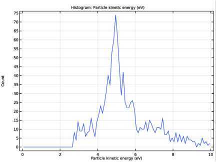
In the Settings window for 1D Plot Group, type Ion Energy Distribution Function in the Label text field.
3
Locate the Data section. From the Dataset list, choose Particle 1.
4
From the Time selection list, choose Last.
Histogram 1
1
Right-click Ion Energy Distribution Function and choose Histogram.
2
In the Settings window for Histogram, click Replace Expression in the upper-right corner of the Expression section. From the menu, choose Model>Component 1>Charged Particle Tracing>Velocity and energy>cpt.Ep - Particle kinetic energy - J.
3
Locate the Expression section. From the Unit list, choose eV.
4
Locate the Bins section. From the Entry method list, choose Limits.
5
Click Range.
6
In the Range dialog box, choose Number of values from the Entry method list.
7
In the Start text field, type 0.
8
In the Stop text field, type 10.
9
In the Number of values text field, type 101.
10
Click Replace.
11
In the Ion Energy Distribution Function toolbar, click Plot. The resulting plot should look like Figure 2.