Electrodynamics of a Power Switch

Electrodynamics of a Power Switch — Multibody Version

Events such as overcurrent or overload can seriously damage electrical circuits or power lines. A possible solution to this problem is the implementation of circuit breakers in the form of automatic electrical switches, which mechanically interrupt the current flow by moving a plunger as soon as a defect is detected. In contrast to a fuse, which has to be replaced after its activation, a circuit breaker can be reset.

Circuit breakers can be classified according to features like voltage rating, construction type, structural features, and interruption technique. The main purpose of this model is to illustrate the working principle and some possible solutions for modeling one class of circuit breakers: magnetic power switches, electromechanical devices in which iron plungers are moved by means of the magnetic attraction exerted by current flowing in coils. Turning off the driving current resets the switch to the initial state. Similar technology is present also in electrovalves and many other magnetic actuators.

The model includes the rigid body dynamics under the influence of magnetic forces, induced currents, and spring/constraint arrangements that keep the plunger in its equilibrium position.

This model requires the AC/DC Module and the Multibody Dynamics Module.

Model Definition

The geometry of the electromechanical device is shown in Figure 1. Two bulk E-shaped iron cores are separated by an air gap. A copper coil is placed on the central leg of the lower E-core, which is kept fixed. As current flows in the coil, an attractive force is exerted on the upper E-core (the moving plunger), which is held in place by a prestressed spring. When the force reaches a threshold value, the plunger moves towards the lower E-core, closing the air gap. The model illustrates how to properly simulate the movement and the closing time, which depends on the spring stiffness.

Figure 1: Geometry of the switch.

The geometry is built using COMSOL Multiphysics’ CAD tools and taking advantage of parameterized Geometry Parts, allowing a finer control on the geometry. Due to the symmetry of the device, it is possible to represent only a quarter of the geometry. Figure 2 shows the simulation geometry, complete with size specifications, which are added as model parameters in COMSOL Multiphysics. In order to compute the electromagnetic fields, the power switch is embedded in an air domain.

Figure 2: Switch specifications.

The model solves a preprocessing study to compute the parameterization of the air gap and the coil direction, as detailed in the following sections, then a main Time Dependent study step from t = 0 s to t = 1 s.

Physics Interfaces

This model uses the Magnetic Fields and Multibody Dynamics interfaces coupled to the Moving Mesh, which allows computing magnetic fields in a geometry that changes with time, due to the closure of the air gap. The Magnetic Fields interface computes the time-dependent magnetic field generated by the coil, the current densities induced in the coils and their magnetic effects. A Coil feature using a homogenized multi-turn model is used for the excitation. The direction of the current flow in the coil is computed automatically in a Coil Geometry Analysis study step. The attractive force acting on the moving domain is computed using a Force Calculation feature. Plunger dynamics is described using Rigid Domain node in the Multibody Dynamics interface. The attractive force acting on the moving domain is modeled as an applied force on the rigid plunger with a given mass.

To improve the stability of the solution in presence of nonlinear magnetic materials, linear elements are used for the discretization of the magnetic vector potential.

Mesh Deformation

During the switching process, the plunger moves rigidly in the vertical direction, while the lower core remains fixed. The mesh in the air gap must then be deformed consistently to accommodate this movement. This is taken care of by the Yeoh smoother.

In order to avoid complete collapse of the mesh, displacement is limited to be at most 90% of the initial air gap, with a marginal impact on the results. This model is set up in order to consider an elastic but highly damped collision between the plunger and fixed core. It is achieved using the locking functionality available in the node in the Multibody Dynamics interface. An alternative solution to model the complete collapse of gap is to use a Stop Condition in the solver sequence, continuing the simulation with a geometry without the gap, or by means of the Events interface.

Results and Discussion

Different stages can be identified in the transient analysis. During the first 45 ms of the simulation the current grows but the electromagnetic attractive force is not enough to overcome the opposing spring force. In the interval between 45 ms and 85 ms the electromagnetic force increases further and the plunger starts to translate downward, toward the iron core; once it reaches this new position it stops its movement. During this stage the current decreases due to the inductance changing, reaching its minimum value with the closing of the air gap. When the plunger and core make contact, a new stationary RL circuit is created. The current starts to increase again with a slope depending on the new characteristic time of the device.

Figure 3 and Figure 4 show the magnetic fields on symmetry planes when the gap is still open (Figure 3) and at a time where the gap is closed (Figure 4). In both cases, it is evident that induced eddy currents are screening the interior of the core from the field. These currents are limited to a region as large as the skin depth, resolved by the boundary layer mesh.

Figure 3: Magnetic flux density norm at t = 0.05 s, when the gap is open.

Figure 4: Magnetic flux density norm at t = 0.1 s, when the gap is closed.

Figure 5 shows the evolution of magnetic field streamlines at different instants of the simulation. The top-left image refers to a time instant in which the spring is still prestressed. As the magnetic force increases, it starts to compress the spring (top right) until it reaches its maximum compression (lower-left). Well before the final time of the simulation, the spring is completely compressed and the induced currents in the core have decayed (lower-right).

Figure 5: Evolution of current density (surface) and magnetic flux density (streamlines) at different times.

Figure 6 shows the core losses in the device due to induced current density. This information may be relevant in order to predict possible overheating of the device.

Figure 6: Core losses due to induced currents at different time instants.

A series of 1D plots are also created to highlight the dynamics of the magnetic switch, before, during, and after plunger motion.

•

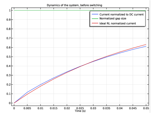
Before plunger motion: Figure 7 shows the first stage of the simulation, when the spring is not yet compressed. Blue and green lines represent normalized currents and gap size respectively. Red line is an exponential fit for the RL current dynamics of the initially non-moving inductor — the response of an ideal system.

•

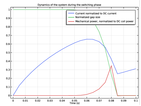
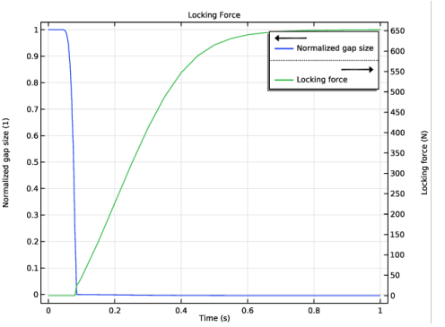
During plunger motion: the compression of the spring and the resulting closure of the gap are visualized in Figure 8. Normalized currents and gap size are represented by blue and green lines respectively, the red line showing instead the mechanical power (which is nonzero only during the motion of the plunger).

•

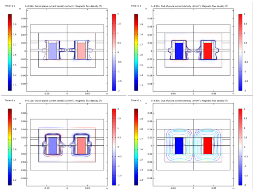
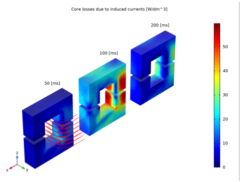
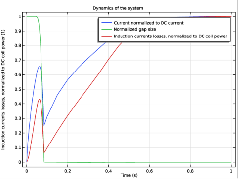
After plunger motion: Figure 9 refers to the last stage of simulation, when the spring is completely compressed. The red line shows the induction losses in the core, which are significant during the movement of the plunger. Depending on the details of the device and the desired performance, this aspect may need to be taken into account during the design process. After the movement is completed, the current starts increasing again as expected in a (nonlinear) RL circuit.

Figure 7: Magnetic flux density norm at t = 0.1 s, when the gap is closed.

Figure 8: Magnetic flux density norm at t = 0.1 s, when the gap is closed.

Figure 9: Magnetic flux density norm at t = 0.1 s, when the gap is closed.

It is worth recalling that blue and green curves in Figure 7, Figure 8, and Figure 9 are representing the same physical quantities, respectively the normalized current and the normalized gap size. The reason why they look different is the limit of the x axis (time scale). Figure 10 shows the variation of locking force with time.

Figure 10: Variation of locking force and gap with time.

ACDC_Module/Motors_and_Actuators/power_switch_multibody

Modeling Instructions

From the menu, choose .

New

In the window, click .

Model Wizard

In the window, click .

In the tree, select .

Click .

In the tree, select .

Click .

In the tree, select .

Click .

Global Definitions

Parameters 1

Import the geometric and physical parameters from an external file.

In the window, under click .

In the window for , locate the section.

Click .

Browse to the model’s Application Libraries folder and double-click the file power_switch_multibody_parameters.txt.

In order to draw the parameterized geometry of the solid parts, create two 2D , one for the core projection and one for the coil. These parts will be successively combined in a third 3D part.

Part 1

In the window, right-click and choose .

In the window for , type Core Section in the text field.

The core section is made up of six rectangles.

Right-click and choose six times, entering the following settings in each node:


Name	Width	Height	xw	yw
Rectangle 1 (r1)	l1	h1	0	h1
Rectangle 2 (r2)	l1+g1+d1+g2+l2	l3	0	-h1-l3
Rectangle 3 (r3)	l2	h1	l1+g1+d1+g2	-h1
Rectangle 4 (r4)	l1	h2	0	d0
Rectangle 5 (r5)	l1+g1+d1+g2+l2	l4	0	d0+h2
Rectangle 6 (r6)	l2	h2	l1+g1+d1+g2	d0

Proceed to create the geometry part for the coil.

Part 2

Right-click and choose .

In the window for , type Coil Section in the text field.

Rectangle 1 (r1)

In the toolbar, click .

In the window for , locate the section.

In the text field, type d1.

In the text field, type l5.

Locate the section. In the text field, type l1+g1.

Circle 1 (c1)

In the toolbar, click .

In the window for , locate the section.

In the text field, type g1+d1.

In the text field, type 90.

Locate the section. In the text field, type l1.

In the text field, type l5.

Click to expand the section. In the table, enter the following settings:


Layer name	Thickness (m)
Layer 1	d1

Rectangle 2 (r2)

In the toolbar, click .

In the window for , locate the section.

In the text field, type l1.

In the text field, type d1.

Locate the section. In the text field, type l5+g1.

Click the button in the toolbar.

Click .

Delete Entities 1 (del1)

In the window, right-click and choose .

In the window for , locate the section.

From the list, choose .

On the object , select Domain 1 only.

Click .

Global Definitions

Create a three-dimensional geometry part for the solid object, combining the two previously created parts.

Part 3

In the window, under right-click and choose .

In the window for , type Solid Parts in the text field.

Work Plane 1 (wp1)

In the toolbar, click .

In the window for , locate the section.

From the list, choose .

Plane Geometry

In the window, click .

Work Plane 1 (wp1)>Core Section 1 (pi1)

In the toolbar, click and choose .

Work Plane 1 (wp1)

In the window, click .

Extrude 1 (ext1)

In the toolbar, click .

In the window for , locate the section.

In the table, enter the following settings:


Distances (m)
l5

Select the check box.

Work Plane 2 (wp2)

In the toolbar, click .

In the window for , locate the section.

In the text field, type -h1.

Plane Geometry

In the window, click .

Work Plane 2 (wp2)>Coil Section 1 (pi1)

In the toolbar, click and choose .

Work Plane 2 (wp2)

In the window, click .

Extrude 2 (ext2)

In the toolbar, click .

In the window for , locate the section.

In the table, enter the following settings:


Distances (m)
d2

In the toolbar, click .

Click the button in the toolbar.

Now create the actual simulation geometry. Start by creating an instance of the three-dimensional geometry part just added. After that, several other solid parts have to be drawn in order to partition properly the air domain surrounding the coil and the core. Refer to the saved .mph file to see a possible parameterized partitioning. The purpose of partitioning the air gap is to minimize as much as possible the distortion of the mesh during the deformation.

Geometry 1

Solid Parts 1 (pi1)

In the toolbar, click and choose .

Right-click and choose .

In order to have a robust geometric parameterization, create a number of nodes.

In the toolbar, use the buttons to create nodes according to the following table:


Selection label	Selection type	Entity level	Entity numbers/Selection settings
Deformed Domains	Explicit, sel1	domain	4, 7, 9-11, 14, 16-19, 23-25, 27-29, 31-34, 36-39, 41
Plunger	Explicit, sel2	domain	5-6, 12, 20-21, 42-43
Fixed Domains	Explicit, sel3	domain	1-3, 8, 13, 15, 22, 26, 30, 35, 40
Ext. Boundaries to Deformed Domains	Adjacent, adj1	domain	sel1, exterior boundaries
Ext. Boundaries to Plunger	Adjacent, adj2	domain	sel2, exterior boundaries
Ext. Boundaries to Fixed Domains	Adjacent, adj3	domain	sel3, exterior boundaries
Fixed Boundaries at Plunger	Intersection	boundary	adj1, adj3
Top Boundary	Explicit, sel4	boundary	22
Fixed Boundaries	Union, uni1	boundary	int1, sel4
Moving Boundaries	Intersection, int2	boundary	adj1, adj2
Nonlinear Core	Explicit, sel5	domain	2-3, 5-6, 40, 42
Ext. Boundaries to Nonlinear Core	Adjacent, adj4	domain	sel5, exterior boundaries
Coil Domain	Explicit, sel6	domain	13, 30, 35

Materials

Next, add the materials — air, a coil material, and soft iron for the coil. For air, use a small and finite conductivity in order to be able to solve using the same formulation used in the conductors.

Material 1 (mat1)

In the window, under right-click and choose .

In the window for , type Air in the text field.

Locate the section. In the table, enter the following settings:


Property	Variable	Value	Unit	Property group
Relative permeability	mur_iso ; murii = mur_iso, murij = 0	1	1	Basic
Electrical conductivity	sigma_iso ; sigmaii = sigma_iso, sigmaij = 0	1	S/m	Basic
Relative permittivity	epsilonr_iso ; epsilonrii = epsilonr_iso, epsilonrij = 0	1	1	Basic

Material 2 (mat2)

Right-click and choose .

In the window for , type Coil Material in the text field.

Locate the section. From the list, choose .

Locate the section. In the table, enter the following settings:


Property	Variable	Value	Unit	Property group
Relative permeability	mur_iso ; murii = mur_iso, murij = 0	1	1	Basic
Electrical conductivity	sigma_iso ; sigmaii = sigma_iso, sigmaij = 0		S/m	Basic
Relative permittivity	epsilonr_iso ; epsilonrii = epsilonr_iso, epsilonrij = 0	1	1	Basic

Add Material

In the toolbar, click to open the window.

Go to the window.

In the tree, select .

Click .

In the toolbar, click to close the window.

Materials

Soft Iron (With Losses) (mat3)

In the window for , locate the section.

From the list, choose .

Mesh 1

Move now to the mesh setup, using a setting for all domains that will later be overwritten in specific parts of the geometry.

In the window, under click .

In the window for , locate the section.

From the list, choose .

Free Triangular 1

Right-click and choose .

Select Boundaries 12, 29, 54, 64, 84, 97, 117, 144, 160, and 174 only.

Size 1

Right-click and choose .

Select Boundaries 12, 29, 54, 84, 97, 117, 144, and 160 only.

In the window for , click to expand the section.

Locate the section. Click the button.

Locate the section. Select the check box.

In the associated text field, type d0*0.5.

Select the check box.

In the associated text field, type 1.2.

Swept 1

In the window, right-click and choose .

In the window for , locate the section.

From the list, choose .

Select Domains 4, 9, 16, 19, 23, 27, 32, 37, and 41 only.

Distribution 1

Right-click and choose .

In the window for , locate the section.

In the text field, type 2.

Swept 2

In the window, right-click and choose .

In the window for , locate the section.

From the list, choose .

Select Domains 10, 17, 24, 28, 33, and 38 only.

Distribution 1

Right-click and choose .

Free Triangular 2

In the window, right-click and choose .

Select Boundaries 47, 112, and 135 only.

Swept 3

Right-click and choose .

In the window for , locate the section.

From the list, choose .

Select Domains 11, 14, 18, 25, 29, 31, 34, 36, and 39 only.

Distribution 1

Right-click and choose .

In the window for , locate the section.

In the text field, type 2.

Free Tetrahedral 1

In the window, right-click and choose .

Use a boundary layer mesh to resolve the skin depth inside the core.

Boundary Layers 1

Right-click and choose .

In the window for , locate the section.

From the list, choose .

Boundary Layer Properties

Select the boundaries interior to the geometry and adjacent to the nonlinear core. The easiest way to do this is as follows:

In the window, click .

From the list box, choose .

Deselect the boundaries exterior to the geometry, leaving only the interior boundaries.

In the window for , locate the section.

In the text field, type 7.

In the text field, type 1.4.

From the list, choose .

In the text field, type 0.2[mm].

Click .

Definitions

Deforming Domain 1

In the toolbar, click and choose .

In the window for , locate the section.

From the list, choose .

Locate the section. In the C2 text field, type 100.

Prescribed Normal Mesh Displacement 1

In the toolbar, click and choose .

Select Boundaries 10, 11, 19, 20, 27, 30, 33, 45, 52, 55, 58, 62, 74, 78, 83, 86, 89, 134, 143, 146, 149, 159, 173, 186, 190, and 191 only.

Prescribed Mesh Displacement 1

In the toolbar, click and choose .

In the window for , locate the section.

From the list, choose .

Prescribed Mesh Displacement 2

In the window, right-click and choose .

In the window for , locate the section.

From the list, choose .

Locate the section. Specify the dx vector as


0	X
0	Y
disp	Z

Magnetic Fields (mf)

In the window, under click .

In the window for , click to expand the section.

From the list, choose .

Coil 1

In the toolbar, click and choose .

In the window for , locate the section.

From the list, choose .

Locate the section. From the list, choose .

From the list, choose .

In the Vcoil text field, type 10[V].

Locate the section. In the N text field, type filling*d1*d2/a_coil.

In the acoil text field, type a_coil.

Geometry Analysis 1

In the window, expand the node.

In the window for , locate the section.

Find the subsection. In the FL text field, type 4.

Input 1

In the window, expand the node, then click .

Select Boundary 129 only.

Output 1

In the window, right-click and choose .

Select Boundary 40 only.

Ampère’s Law 2

In the toolbar, click and choose .

In the window for , locate the section.

From the list, choose .

Locate the section. From the list, choose .

Force Calculation 1

In the toolbar, click and choose .

Select Domains 5, 6, and 42 only.

Gauge Fixing for A-field 1

In the toolbar, click and choose .

Multibody Dynamics (mbd)

In the window, under click .

In the window for , locate the section.

From the list, choose .

Rigid Domain 1

In the toolbar, click and choose .

In the window for , locate the section.

From the list, choose .

Locate the section. From the ρ list, choose . In the window, click .

Mass and Moment of Inertia 1

In the toolbar, click and choose .

In the window for , locate the section.

In the m text field, type mass.

Applied Force 1

In the window, right-click and choose .

In the window for , locate the section.

Specify the F vector as


0	x
0	y
min(mf.Forcez_0+k0*(x0-disp),0)	z

Prismatic Joint 1

In the toolbar, click and choose .

In the window for , locate the section.

From the list, choose .

In the window for , locate the section.

From the list, choose .

In the window, click .

In the window for , locate the section.

Specify the e0 vector as


0	x
0	y
1	z

Locking 1

In the toolbar, click and choose .

In the window for , locate the section.

In the umin text field, type -maxdisp.

In the window for , locate the section.

From the list, choose .

In the window, click .

In the window for , locate the section.

In the pu1 text field, type (0.01*mbd.prj1.lk1.Eequ)*mbd.diag/10.

In the pu2 text field, type mbd.prj1.lk1.p_u1*10[ms]/50.

Definitions

Variables 1

In the window, under right-click and choose .

In the window for , locate the section.

In the table, enter the following settings:


Name	Expression	Unit	Description
disp	mbd.rd1.w	m	Plunger displacement
vel	mbd.rd1.wt	m/s	Velocity of plunger

The first study consists of a preprocessing step to solve which is needed in order to compute the direction of the coil.

Study 1

In the window, click .

In the window for , type Study 1 (Preprocessing) in the text field.

Locate the section. Clear the check box.

In the toolbar, click .

Results

3D Plot Group 1

In the toolbar, click and choose .

In the window for , type Preprocessing: Air Gap Parameterization and Coil Direction in the text field.

Click to expand the section. From the list, choose .

In the text area, type Preprocessing: Air Gap Parameterization and Coil Direction.

Volume 1

Right-click and choose .

In the window for , locate the section.

In the text field, type 1.

Filter 1

Right-click and choose .

In the window for , locate the section.

In the text field, type y<x.

In the toolbar, click .

Streamline 1

In the window, right-click and choose .

Select Boundary 129 only.

In the window for , click in the upper-right corner of the section. From the menu, choose .

Locate the section. Find the subsection. From the list, choose .

Find the subsection. From the list, choose .

In the toolbar, click .

Click the button in the toolbar.

Root

Now create the main study containing the step. Specify that the step must use the values computed in the preprocessing study.

Add Study

In the toolbar, click to open the window.

Go to the window.

Find the subsection. In the tree, select .

Click in the window toolbar.

In the toolbar, click to close the window.

Study 2

In the window, click .

In the window for , type Study 2 (Time Dependent) in the text field.

Step 1: Time Dependent

In the window, under click .

In the window for , locate the section.

In the text field, type range(0,0.005,0.1) range(0.15,0.05,1).

Click to expand the section. Find the subsection. From the list, choose .

From the list, choose .

Solution 2 (sol2)

In the toolbar, click .

Apply typical solver settings for strongly nonlinear problems.

In the window, expand the node.

In the window, expand the node, then click .

In the window for , locate the section.

From the list, choose .

In the text field, type 1e-3.

In the window, click .

In the window for , locate the section.

From the list, choose .

In the window, click .

In the window for , locate the section.

From the list, choose .

In the window, expand the node.

Right-click and choose .

In the window for , locate the section.

From the list, choose .

In the window, click .

In the window for , click to expand the section.

Find the subsection. From the list, choose .

From the list, choose .

Click to expand the section. From the list, choose .

In the text field, type 0.01.

Right-click and choose .

In the window for , locate the section.

From the list, choose .

Click to expand the section. From the list, choose .

In the toolbar, click . The solution process will need about 50 minutes on a typical workstation.

Results

Modify the previously generated plot to visualize the normalized displacement in the moving mesh regions. It is possible to verify that the material frame representation of this quantity does not depend significanly on the time after the moving anchor has moved away from its rest position.

Volume 1

In the window, under click .

In the window for , locate the section.

From the list, choose .

Locate the section. In the text field, type (z-Z)/disp.

Selection 1

Right-click and choose .

In the window for , locate the section.

From the list, choose .

Multislice 1

In the window, expand the node, then click .

In the window for , locate the section.

Find the subsection. In the text field, type 0.

Find the subsection. From the list, choose .

Find the subsection. In the text field, type 0.

Magnetic Flux Density Norm (mf)

In the window, click .

In the window for , locate the section.

From the list, choose .

In the toolbar, click .

The generated plot shows the magnetic fields on the symmetry planes at the last time step, when the gap is closed and the induction currents have decayed.

Locate the section. From the list, choose .

In the toolbar, click .

The generated plot shows the magnetic fields on the symmetry planes at a time when the gap was still open.

In the window, click .

In the window for , locate the section.

From the list, choose .

In the toolbar, click .

The generated plot shows the magnetic fields on the symmetry planes at a time step in which the gap is closed and induction currents are screening the interior of the core to the field.

Datasets

A 2D section of the complete geometry can be produced with the following instructions.

Mirror 3D 1

In the toolbar, click and choose .

In the window for , locate the section.

From the list, choose .

Cut Plane 1

In the toolbar, click .

In the window for , locate the section.

From the list, choose .

Locate the section. From the list, choose .

2D Plot Group 6

In the toolbar, click .

In the window for , click to expand the section.

In the text field, type Current Density and Magnetic Flux Lines.

Locate the section. From the list, choose .

In the text area, type t=0.01s: Out-of-plane current density (A/mm<sup>2</sup>), Magnetic flux density (T).

Locate the section. From the list, choose .

Surface 1

Right-click and choose .

In the window for , locate the section.

In the text field, type mf.Jy.

In the field, type A/mm^2.

Click to expand the section. Select the check box.

In the text field, type -2.

In the text field, type 2.

Locate the section. From the list, choose .

In the toolbar, click .

The plot shows the currents perpendicular to the xz -plane, simply mirrored. Use a side indicator variable to provide the correct sign for the currents.

Mirror 3D 1

In the window, click .

In the window for , click to expand the section.

Select the check box.

Surface 1

In the window, click .

In the window for , locate the section.

In the text field, type mf.Jy*sign(mir1x).

In the toolbar, click .

Current Density and Magnetic Flux Lines

Vector quantities are automatically correct when inherited from a mirror dataset.

Streamline 1

In the window, right-click and choose .

In the window for , locate the section.

In the text field, type mf.Bx.

In the text field, type mf.Bz.

Locate the section. From the list, choose .

In the text field, type range(-0.018,0.004,0.018).

In the text field, type 0.

Click to expand the section. In the text field, type 0.1.

Color Expression 1

Right-click and choose .

In the window for , click to expand the section.

Select the check box.

In the text field, type 2.

Current Density and Magnetic Flux Lines

In the window, click .

In the window for , locate the section.

From the list, choose .

Locate the section. From the list, choose .

In the toolbar, click .

The plot shows the field and geometry configuration at a time instant in which the gap is still open. Use the list box to visualize the solution at different time instants.

Create a plot showing the losses in the core at different times, in the same 3D visualization.

3D Plot Group 7

In the toolbar, click and choose .

In the window for , locate the section.

From the list, choose .

In the text field, type Core Losses.

Locate the section. From the list, choose .

In the text area, type Core losses due to induced currents [W/dm^3].

Locate the section. Clear the check box.

Streamline 1

Right-click and choose .

In the window for , locate the section.

In the text field, type mf.Jx.

In the text field, type mf.Jy.

In the text field, type mf.Jz.

Select Boundary 129 only.

Volume 1

In the window, right-click and choose .

In the window for , locate the section.

From the list, choose .

Locate the section. In the text field, type mf.Qrh.

In the field, type W/dm^3.

Locate the section. From the list, choose .

Selection 1

Right-click and choose .

In the window for , locate the section.

From the list, choose .

Volume 2

In the window, under right-click and choose .

In the window for , locate the section.

From the list, choose .

Deformation 1

Right-click and choose .

In the window for , locate the section.

In the text field, type -0.1.

In the text field, type 0.

Locate the section. Select the check box.

In the associated text field, type 1.

Volume 2

In the window, click .

In the window for , click to expand the section.

From the list, choose .

Volume 3

Right-click and choose .

In the window for , locate the section.

From the list, choose .

Deformation 1

In the window, expand the node, then click .

In the window for , locate the section.

In the text field, type -0.2.

Annotation 1

In the window, right-click and choose .

In the window for , locate the section.

In the text field, type 50 [ms].

Locate the section. In the text field, type 0.03.

In the text field, type 0.07.

Locate the section. Clear the check box.

Annotation 2

Right-click and choose .

In the window for , locate the section.

In the text field, type 100 [ms].

Locate the section. In the text field, type -0.07.

In the text field, type 0.07.

Locate the section. Clear the check box.

Annotation 3

Right-click and choose .

In the window for , locate the section.

In the text field, type 200 [ms].

Locate the section. In the text field, type -0.17.

In the text field, type 0.07.

Locate the section. Clear the check box.

Then generate the plot and rotate the view with the mouse to visualize the solution.

Create a first 1D plot to visualize the dynamics at the beginning of the process, when the spring is not yet compressed. Plot the normalized currents, gap size, and an exponential fit for the RL current dynamics in a charging inductor.

1D Plot Group 8

In the toolbar, click and choose .

In the window for , type Dynamics, Before Switching in the text field.

Click to expand the section. From the list, choose .

In the text area, type Dynamics of the system, before switching.

Global 1

Right-click and choose .

In the window for , locate the section.

From the list, choose .

In the text field, type range(0,0.005,0.05).

Locate the section. In the table, enter the following settings:


Expression	Unit	Description
mf.ICoil_1*mf.RCoil_1/mf.VCoil_1	1	Current normalized to DC current
1+disp/maxdisp	1	Normalized gap size
1-exp(-t/50[ms])		Ideal RL normalized current

Click to expand the section. In the toolbar, click .

Dynamics, Before Switching

From the first 1D plot, create a second one is to visualize the dynamics of the spring compression. Plot normalized current, gap size, and mechanical power of the moving plunger. Mechanical power is directly linked to the change in inductance, in turn forcing the current to decrease as the gap closes.

Dynamics, Before Switching 1

In the window, right-click and choose .

In the window for , type Dynamics During Switching in the text field.

Locate the section. In the text area, type Dynamics of the system during the switching phase.

Global 1

In the window, expand the node, then click .

In the window for , locate the section.

In the text field, type range(0,0.005,0.1).

Locate the section. In the table, enter the following settings:


Expression	Unit	Description
mf.ICoil_1*mf.RCoil_1/mf.VCoil_1	1	Current normalized to DC current
1+disp/maxdisp	1	Normalized gap size
4massd(vel,t)vel/at(1,mf.ICoil_1mf.VCoil_1)	1	Mechanical power, normalized to DC coil power