PDF

Magnetically Permeable Sphere in a Static Magnetic Field
Introduction
A sphere of relative permeability greater than unity is exposed to a spatially uniform static background magnetic field. Two formulations are used to solve this problem, and the differences between these are discussed. The field strength inside the sphere is computed and compared against the analytic solution.
Figure 1: A magnetically permeable sphere in a spatially uniform, static background magnetic field. The sphere at the center is surrounded by air, and enclosed in a region of Infinite Elements.
Model Definition
Figure 1 shows the model setup, with a 0.25 mm diameter sphere placed in a spatially uniform background magnetic field of strength 1 mT. The computational model consists of three concentric spheres. The innermost is the permeable sphere, the surrounding spherical shell volume represents free space, and the outside shell volume represents a region extending to infinity, modeled with an Infinite Element Domain. When using Infinite Element Domain features, the boundary condition on the outside of the modeling domain does not affect the solution.
The relative permeability of the sphere is varied from μr = 2 to μr = 1000. The analytic solution for the field inside a permeable sphere exposed to a uniform magnetic field is:
Where B0 is the background magnetic field.
There are two ways in which this problem can be formulated. The scalar potential formulation, used in the Magnetic Fields, No Currents interface, solves the magnetic flux conservation equation:
a partial differential equation for the magnetic scalar potential field, Vm:
where the background field is specified in terms of the H-field, Hb. The B-field is then computed from the H-field: B = μrμ0H. The magnetic field is in turn computed from the gradient of the magnetic scalar potential. Because the governing equation evaluates the gradients of a scalar field, the Lagrange element formulation is used. In this formulation, the background field and boundary conditions for this problem are specified purely in terms of derivatives of the Vm field, and the solution is unique up to a constant. To remove this indeterminacy, the value of the magnetic scalar potential must be constrained at one point in the model, to fix the value of the constant.
The vector potential formulation, used in the Magnetic Fields interface, solves an equation for the magnetic vector potential, A:
Where the B-field is the curl of the (A + Ab) field. In this approach, the background field and boundary conditions are specified directly in terms of the A-field. Here, the governing equation takes the curl of a vector valued field, and this problem is solved using a Curl element formulation. This formulation does not require as fine of a mesh as the Lagrange element formulation to achieve the same accuracy.
Results and Discussion
Figure 2 plots the magnetic field for the Magnetic Fields, No Currents interface formulation, and Figure 3 shows the results computed using the Magnetic Fields interface formulation, both for the μr = 1000 case. The fields in the Infinite Element region are not plotted, as these do not have any physical significance.
Figure 4 shows the field enhancement versus the permeability for both cases, along with the analytic solution. The relative difference is plotted in Figure 5. In the limit as the mesh is refined the solutions agree within numerical precision.
There are some differences between the two formulations. In this case, the Magnetic Fields interface slightly underestimates the field strength, while the Magnetic Fields, No Current interface overestimates it. The agreement with the analytic solution for both formulations improves with increasing mesh refinement. Although the Magnetic Fields, No Currents interface require a finer mesh for approximately the same level of accuracy, it does use less total memory. Its drawback is that it cannot be used to model situations where there is any current flowing in the model, or any variation with respect to time.
Figure 2: The magnetic field for the Magnetic Fields, No Currents interface.
Figure 3: The magnetic field for the Magnetic Fields interface.
Figure 4: Comparison of numerical results to analytic result.
Figure 5: Relative difference compared to the analytic solution.
Application Library path: ACDC_Module/Tutorials/permeable_sphere_static_bfield
Modeling Instructions
From the File menu, choose New.
New
In the New window, click Model Wizard.
Model Wizard
1
In the Model Wizard window, click 3D.
2
In the Select Physics tree, select AC/DC>Magnetic Fields, No Currents>Magnetic Fields, No Currents (mfnc).
3
Click Add.
4
Click Study.
5
In the Select Study tree, select General Studies>Stationary.
6
Click Done.
Geometry 1
1
In the Model Builder window, under Component 1 (comp1) click Geometry 1.
2
In the Settings window for Geometry, locate the Units section.
3
From the Length unit list, choose mm.
Global Definitions
Parameters 1
1
In the Model Builder window, under Global Definitions click Parameters 1.
2
In the Settings window for Parameters, locate the Parameters section.
3
Geometry 1
Sphere 1 (sph1)
Create a sphere with two layers plus an inner core. The outermost layer represents the exterior air region, scaled using the Infinite Element Domain, the median layer is the unscaled air domain, and the core represents the permeable sphere.
1
In the Geometry toolbar, click Sphere.
2
In the Settings window for Sphere, locate the Size section.
3
In the Radius text field, type r0*3.
4
Click to expand the Layers section. In the table, enter the following settings:
5
Click Build All Objects.
6
Click the Wireframe Rendering button in the Graphics toolbar.
7
Click the Zoom In button in the Graphics toolbar.
Definitions
Create a set of selections before setting up the physics. First, create a selection for the Infinite Element Domain feature.
Explicit 1
1
In the Definitions toolbar, click Explicit.
2
3
Right-click Explicit 1 and choose Rename.
4
In the Rename Explicit dialog box, type Infinite Element domains in the New label text field.
5
Add a selection for the analysis domains. This is the complement of the Infinite Element domains selection.
Complement 1
1
In the Definitions toolbar, click Complement.
2
In the Settings window for Complement, locate the Input Entities section.
3
Under Selections to invert, click Add.
4
In the Add dialog box, select Infinite Element domains in the Selections to invert list.
5
6
Right-click Complement 1 and choose Rename.
7
In the Rename Complement dialog box, type Analysis domain in the New label text field.
8
Infinite Element Domain 1 (ie1)
1
In the Definitions toolbar, click Infinite Element Domain.
2
In the Settings window for Infinite Element Domain, locate the Domain Selection section.
3
From the Selection list, choose Infinite Element domains.
4
Locate the Geometry section. From the Type list, choose Spherical.
View 1
Suppress some domains to get a better view when setting up the physics and reviewing the meshed results.
Hide for Physics 1
1
In the Model Builder window, right-click View 1 and choose Hide for Physics.
2
Magnetic Fields, No Currents (mfnc)
Set up the first physics — Magnetic Fields, No Currents. Begin by specifying the background magnetic field.
1
In the Model Builder window, under Component 1 (comp1) click Magnetic Fields, No Currents (mfnc).
2
In the Settings window for Magnetic Fields, No Currents, locate the Background Magnetic Field section.
3
From the Solve for list, choose Reduced field.
4
Specify the Hb vector as
Add a constraint point for the magnetic scalar potential.
Zero Magnetic Scalar Potential 1
1
In the Physics toolbar, click Points and choose Zero Magnetic Scalar Potential.
2
Materials
Assign the material properties. First, use air for all domains.
Add Material
1
In the Home toolbar, click Add Material to open the Add Material window.
2
Go to the Add Material window.
3
4
Click Add to Component in the window toolbar.
5
In the Home toolbar, click Add Material to close the Add Material window.
Materials
Override the core sphere with a permeable material.
Material 2 (mat2)
1
In the Model Builder window, under Component 1 (comp1) right-click Materials and choose Blank Material.
2
3
In the Settings window for Material, locate the Material Contents section.
4
The Physics-controlled mesh setting creates a swept mesh for the Infinite Element Domain.
Mesh 1
1
In the Model Builder window, under Component 1 (comp1) click Mesh 1.
2
In the Settings window for Mesh, click Build All.
Study 1
Step 1: Stationary
1
In the Model Builder window, under Study 1 click Step 1: Stationary.
2
In the Settings window for Stationary, click to expand the Study Extensions section.
3
Select the Auxiliary sweep check box.
4
Click Add.
5
6
In the Home toolbar, click Compute.
Results
Datasets
The default plot shows the magnetic flux density for all domains. Add a selection to the current solution to visualize only the Analysis domain.
Selection
1
In the Model Builder window, expand the Results>Datasets node.
2
Right-click Study 1/Solution 1 (sol1) and choose Selection.
3
In the Settings window for Selection, locate the Geometric Entity Selection section.
4
From the Geometric entity level list, choose Domain.
5
From the Selection list, choose Analysis domain.
Magnetic Flux Density Norm (mfnc)
Add an arrow plot showing the direction of the magnetic flux density.
Arrow Volume 1
1
In the Model Builder window, right-click Magnetic Flux Density Norm (mfnc) and choose Arrow Volume.
2
In the Settings window for Arrow Volume, locate the Arrow Positioning section.
3
Find the X grid points subsection. In the Points text field, type 20.
4
Find the Y grid points subsection. In the Points text field, type 20.
5
Find the Z grid points subsection. In the Points text field, type 1.
6
In the Magnetic Flux Density Norm (mfnc) toolbar, click Plot.
Compare the plot with Figure 2.
Repeat the analysis with the Magnetic Fields interface.
Add Physics
1
In the Home toolbar, click Add Physics to open the Add Physics window.
2
Go to the Add Physics window.
3
In the tree, select AC/DC>Electromagnetic Fields>Magnetic Fields (mf).
4
Find the Physics interfaces in study subsection. In the table, clear the Solve check box for Study 1.
5
Click Add to Component 1 in the window toolbar.
6
In the Home toolbar, click Add Physics to close the Add Physics window.
Root
In the Model Builder window, click the root node.
Add Study
1
In the Home toolbar, click Add Study to open the Add Study window.
2
Go to the Add Study window.
3
Find the Studies subsection. In the Select Study tree, select General Studies>Stationary.
4
Find the Physics interfaces in study subsection. In the table, clear the Solve check box for Magnetic Fields, No Currents (mfnc).
5
Click Add Study in the window toolbar.
6
In the Home toolbar, click Add Study to close the Add Study window.
Study 2
Step 1: Stationary
Set up the Magnetic Fields interface. Specify the background field in terms of a magnetic vector potential.
Magnetic Fields (mf)
1
In the Model Builder window, under Component 1 (comp1) click Magnetic Fields (mf).
2
In the Settings window for Magnetic Fields, locate the Background Field section.
3
From the Solve for list, choose Reduced field.
4
Specify the Ab vector as
Materials
Material 2 (mat2)
Assign the material properties to the permeable sphere.
1
In the Model Builder window, under Component 1 (comp1)>Materials click Material 2 (mat2).
2
In the Settings window for Material, locate the Material Contents section.
3
Component 1 (comp1)
Add manually a different mesh for the second physics interface starting from the physics induced sequence.
Mesh 2
In the Mesh toolbar, click Add Mesh.
Size
Right-click Mesh 2 and choose Edit Physics-Induced Sequence.
Distribution 1
1
In the Model Builder window, expand the Component 1 (comp1)>Meshes>Mesh 2>Swept 1 node, then click Distribution 1.
2
In the Settings window for Distribution, locate the Distribution section.
3
In the Number of elements text field, type 2.
4
Click Build All.
Study 2
Step 1: Stationary
1
In the Model Builder window, under Study 2 click Step 1: Stationary.
2
In the Settings window for Stationary, click to expand the Mesh Selection section.
3
4
Locate the Study Extensions section. Select the Auxiliary sweep check box.
5
Click Add.
6
7
In the Home toolbar, click Compute.
Results
Selection
1
In the Model Builder window, right-click Study 2/Solution 2 (sol2) and choose Selection.
2
In the Settings window for Selection, locate the Geometric Entity Selection section.
3
From the Geometric entity level list, choose Domain.
4
From the Selection list, choose Analysis domain.
Datasets
Add a Cut Point 3D data set for both physics. At the origin, the numerical and analytical results are evaluated.
Cut Point 3D 1
1
In the Results toolbar, click Cut Point 3D.
2
In the Settings window for Cut Point 3D, locate the Point Data section.
3
In the X text field, type 0.
4
In the Y text field, type 0.
5
In the Z text field, type 0.
Cut Point 3D 2
1
In the Results toolbar, click Cut Point 3D.
2
In the Settings window for Cut Point 3D, locate the Data section.
3
From the Dataset list, choose Study 2/Solution 2 (sol2).
4
Locate the Point Data section. In the X text field, type 0.
5
In the Y text field, type 0.
6
In the Z text field, type 0.
Arrow Volume 1
1
In the Model Builder window, right-click Magnetic Flux Density Norm (mf) and choose Arrow Volume.
2
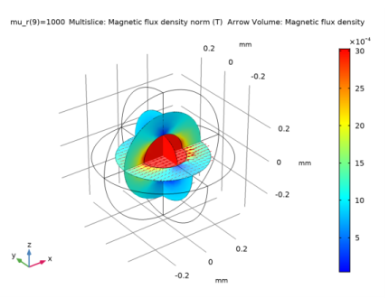
In the Settings window for Arrow Volume, click Replace Expression in the upper-right corner of the Expression section. From the menu, choose Component 1>Magnetic Fields>Magnetic>mf.Bx,mf.By,mf.Bz - Magnetic flux density.
3
Locate the Arrow Positioning section. Find the X grid points subsection. In the Points text field, type 20.
4
Find the Y grid points subsection. In the Points text field, type 20.
5
Find the Z grid points subsection. In the Points text field, type 1.
6
In the Magnetic Flux Density Norm (mf) toolbar, click Plot.
The plot should look like Figure 3.
1D Plot Group 3
1
In the Home toolbar, click Add Plot Group and choose 1D Plot Group.
2
In the Settings window for 1D Plot Group, locate the Axis section.
3
Select the x-axis log scale check box.
Point Graph 1
1
Right-click 1D Plot Group 3 and choose Point Graph.
2
In the Settings window for Point Graph, locate the Data section.
3
From the Dataset list, choose Cut Point 3D 1.
4
Locate the y-Axis Data section. In the Expression text field, type mfnc.normB.
5
Click to expand the Coloring and Style section. Find the Line style subsection. From the Line list, choose None.
6
From the Color list, choose Green.
7
Find the Line markers subsection. From the Marker list, choose Point.
8
From the Positioning list, choose In data points.
Point Graph 2
1
In the Model Builder window, right-click 1D Plot Group 3 and choose Point Graph.
2
In the Settings window for Point Graph, locate the Data section.
3
From the Dataset list, choose Cut Point 3D 1.
4
Locate the y-Axis Data section. In the Expression text field, type B_analytic.
5
Locate the Coloring and Style section. Find the Line style subsection. From the Line list, choose Dotted.
6
From the Color list, choose Black.
Point Graph 3
1
Right-click 1D Plot Group 3 and choose Point Graph.
2
In the Settings window for Point Graph, locate the Data section.
3
From the Dataset list, choose Cut Point 3D 2.
4
Locate the y-Axis Data section. In the Expression text field, type mf.normB.
5
Locate the Coloring and Style section. Find the Line style subsection. From the Line list, choose None.
6
From the Color list, choose Red.
7
Find the Line markers subsection. From the Marker list, choose Diamond.
8
From the Positioning list, choose In data points.
9
In the 1D Plot Group 3 toolbar, click Plot.
1D Plot Group 4
1
In the Home toolbar, click Add Plot Group and choose 1D Plot Group.
2
In the Settings window for 1D Plot Group, locate the Axis section.
3
Select the x-axis log scale check box.
Point Graph 1
1
Right-click 1D Plot Group 4 and choose Point Graph.
2
In the Settings window for Point Graph, locate the Data section.
3
From the Dataset list, choose Cut Point 3D 1.
4
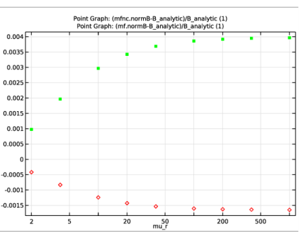
Locate the y-Axis Data section. In the Expression text field, type (mfnc.normB-B_analytic)/B_analytic.
5
Locate the Coloring and Style section. Find the Line style subsection. From the Line list, choose None.
6
From the Color list, choose Green.
7
Find the Line markers subsection. From the Marker list, choose Point.
8
From the Positioning list, choose In data points.
Point Graph 2
1
In the Model Builder window, right-click 1D Plot Group 4 and choose Point Graph.
2
In the Settings window for Point Graph, locate the Data section.
3
From the Dataset list, choose Cut Point 3D 2.
4
Locate the y-Axis Data section. In the Expression text field, type (mf.normB-B_analytic)/B_analytic.
5
Locate the Coloring and Style section. Find the Line style subsection. From the Line list, choose None.
6
From the Color list, choose Red.
7
Find the Line markers subsection. From the Marker list, choose Diamond.
8
From the Positioning list, choose In data points.
9
In the 1D Plot Group 4 toolbar, click Plot.
Compare the resulting plots with Figure 4 and Figure 5.