|
|
|

|
1
|
|
2
|
|
3
|
Click Add.
|
|
4
|
|
5
|
Click Add.
|
|
6
|
Click Study.
|
|
7
|
|
8
|
Click Done.
|
|
1
|
|
2
|
|
1
|
|
2
|
|
3
|
|
4
|
|
5
|
|
6
|
|
7
|
|
8
|
|
1
|
|
2
|
|
3
|
|
4
|
|
5
|
|
6
|
|
7
|
|
8
|
|
9
|
|
1
|
|
2
|
|
3
|
|
4
|
|
5
|
|
6
|
|
7
|
|
8
|
|
1
|
|
2
|
|
3
|
|
4
|
|
5
|
|
6
|
|
7
|
|
8
|
|
9
|
|
1
|
|
2
|
|
3
|
|
4
|
|
5
|
|
6
|
|
7
|
|
8
|
|
9
|
|
10
|
|
1
|
|
2
|
|
3
|
|
4
|
Browse to the model’s Application Libraries folder and double-click the file magnetotellurics_variables.txt.
|
|
1
|
In the Model Builder window, under Component 1 (comp1) right-click Materials and choose Blank Material.
|
|
3
|
|
5
|
|
6
|
|
7
|
Click OK.
|
|
1
|
|
3
|
|
5
|
|
6
|
|
7
|
Click OK.
|
|
1
|
|
3
|
|
5
|
|
6
|
|
7
|
Click OK.
|
|
1
|
|
3
|
|
5
|
|
6
|
|
7
|
Click OK.
|
|
1
|
|
2
|
|
3
|
|
5
|
|
6
|
|
7
|
Click OK.
|
|
1
|
|
2
|
|
3
|
|
5
|
|
6
|
|
7
|
Click OK.
|
|
1
|
|
2
|
|
3
|
|
5
|
|
6
|
|
7
|
Click OK.
|
|
1
|
In the Model Builder window, under Component 1 (comp1) right-click Magnetic Fields (mf) and choose Perfect Magnetic Conductor.
|
|
2
|
|
3
|
|
1
|
|
2
|
|
3
|
|
4
|
|
1
|
In the Model Builder window, under Component 1 (comp1) right-click Magnetic Fields 2 (mf2) and choose Perfect Magnetic Conductor.
|
|
2
|
|
3
|
|
1
|
|
2
|
|
3
|
|
4
|
|
1
|
In the Model Builder window, under Component 1 (comp1) right-click Mesh 1 and choose More Operations>Free Triangular.
|
|
3
|
|
1
|
|
3
|
|
4
|
|
1
|
|
3
|
|
4
|
|
1
|
|
2
|
|
3
|
|
5
|
|
6
|
|
1
|
|
2
|
|
3
|
|
4
|
Locate the Physics and Variables Selection section. In the table, clear the Solve for check box for the Magnetic Fields 2 interface.
|
|
1
|
|
2
|
|
3
|
|
4
|
Locate the Physics and Variables Selection section. In the table, clear the Solve for check box for the Magnetic Fields interface.
|
|
1
|
|
2
|
|
3
|
|
4
|
|
5
|
Locate the Initial Values of Variables Solved For section. From the Method list, choose Initial expression.
|
|
6
|
|
7
|
|
8
|
|
1
|
|
2
|
|
3
|
|
1
|
|
2
|
|
3
|
|
4
|
|
5
|
|
1
|
|
2
|
|
3
|
|
4
|
|
5
|
|
6
|
|
7
|
Click OK.
|
|
1
|
|
2
|
|
3
|
|
1
|
|
2
|
|
3
|
|
4
|
|
5
|
|
6
|
|
7
|
|
8
|
Click OK.
|
|
1
|
|
2
|
|
3
|
|
4
|
|
1
|
|
2
|
|
3
|
|
1
|
|
2
|
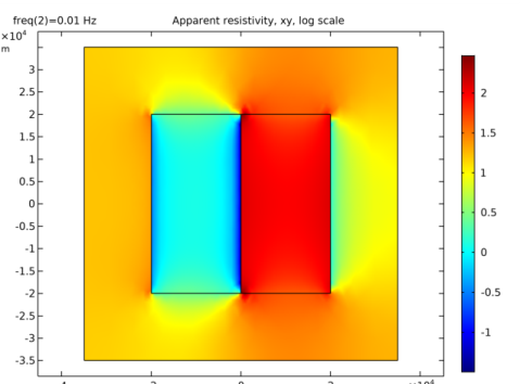
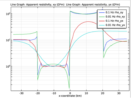
In the Settings window for Line Graph, click Replace Expression in the upper-right corner of the y-axis data section. From the menu, choose Component 1>Definitions>Variables>rho_xy - Apparent resistivity, xy - Ω·m.
|
|
3
|
|
4
|
Click Replace Expression in the upper-right corner of the x-axis data section. From the menu, choose Component 1>Geometry>Coordinate>x - x-coordinate.
|
|
5
|
|
6
|
|
7
|
|
9
|
|
10
|
|
1
|
|
2
|
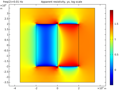
In the Settings window for Line Graph, click Replace Expression in the upper-right corner of the y-axis data section. From the menu, choose Component 1>Definitions>Variables>rho_yx - Apparent resistivity, yx - Ω·m.
|
|
3
|
Locate the Legends section. In the table, enter the following settings:
|
|
4
|
|
1
|
|
2
|
In the Rename 1D Plot Group dialog box, type Apparent resistivity across strike in the New label text field.
|
|
3
|
Click OK.
|
|
1
|
|
2
|
|
1
|
|
2
|
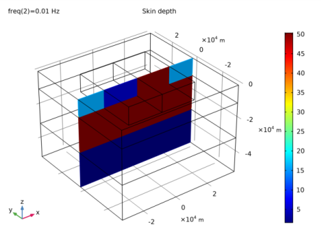
In the Settings window for Slice, click Replace Expression in the upper-right corner of the Expression section. From the menu, choose Component 1>Magnetic Fields>Material properties>mf.deltaS - Skin depth - m.
|
|
3
|
|
4
|
|
5
|
|
1
|
|
2
|
|
3
|
|
4
|
|
5
|
|
6
|
|
7
|
|
8
|
Click OK.
|
|
1
|
|
2
|
|
1
|
|
2
|
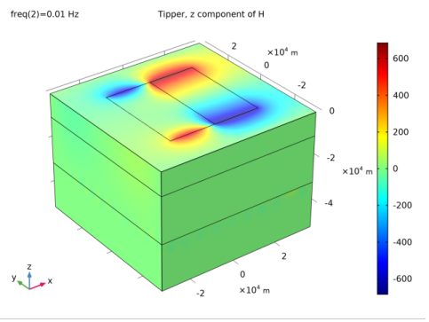
In the Settings window for Surface, click Replace Expression in the upper-right corner of the Expression section. From the menu, choose Component 1>Magnetic Fields>Magnetic>Magnetic field - A/m>mf.Hz - Magnetic field, z component.
|
|
1
|
|
2
|
|
3
|
|
4
|
|
5
|
|
6
|
|
7
|
|
8
|
Click OK.
|