PDF

Inductor in an Amplifier Circuit
Introduction
This example studies a finite element model of an inductor inserted into an electrical amplifier circuit.
Modern electronic systems are very complex and depend heavily on computer aided design in the development and manufacturing process. Common tools for such calculations are based on the SPICE format originally developed at Berkeley University (Ref. 1). The SPICE format consists of a standardized set of models for describing electrical devices — especially semiconductor devices such as transistors, diodes, and thyristors. SPICE also includes a simple, easy-to-read text format for circuit netlists and model parameter specifications. Although the netlist format is essentially the same as it was from the beginning, the set of models and model parameters constantly changes, with new models being added according to the latest achievements in semiconductor device development. When the devices are scaled down, new effects appear that have to be properly modeled. The new models are the result of ongoing research in device modeling.
When an engineer is designing a new electronic component, like a capacitor or an inductor, the SPICE parameters for that device are not known. They are either extracted from finite element tools such as COMSOL Multiphysics or from measurements on a prototype. To speed up the design process it can be convenient to include the finite element model in the SPICE circuit simulation, calculating the device behavior in an actual circuit.
This model takes a simple amplifier circuit and exchanges one of its components with a finite element model of an inductor with a magnetic core. COMSOL Multiphysics calculates the transient behavior of the entire system. Importing a SPICE circuit netlist brings in the circuit elements along with their model parameters and location in the circuit. All elements can be edited in COMSOL Multiphysics, and any pair of nodes can connect to the finite element model.
Model Definition
The inductor model uses the Magnetic Fields interface solving for the magnetic potential A:
where μ0 is the permeability of vacuum, μr the relative permeability, and σ the electrical conductivity.
Because the coil has a large number of turns it is not efficient to model the separate wires and a homogenized formulation, where eddy currents within each wire are neglected, is used for the coil cross section. A dedicated coil feature is used for this purpose.
Connection to a Spice Circuit
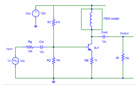
The electrical circuit is a standard amplifier circuit with one bipolar transistor, biasing resistors, input filter, and output filter; see Figure 1.
Figure 1: Circuit diagram.
The input is a sine signal of 1 V and 10 kHz. The following listing shows the SPICE netlist for this circuit:
* BJT Amplifier circuit
.OPTIONS TNOM=27
.TEMP 27
Vin 1 0 sin(0 1 10kHz)
Vcc 4 0 15
Rg 1 2 100
Cin 2 3 10u
R1 4 3 47k
R2 3 0 10k
RE 7 0 1k
Cout 5 6 10u
Rl 6 0 10k
Q1 5 3 7 BJT
.MODEL BJT NPN(Is=15f Ise=15f Isc=0 Bf=260 Br=6.1
+ Ikf=.3 Xtb=1.5 Ne=1.3 Nc=2 Rc=1 Rb=10 Eg=1.11
+ Cjc=7.5p Mjc=.35 Vjc=.75 Fc=.5 Cje=20p Mje=0.4 Vje=0.75
+ Vaf=75 Xtf=3 Xti=3)
.END
A dedicated circuit device is then added in COMSOL Multiphysics to connect the circuit with the inductor model. The model parameters of the transistor do not correspond to a real device, but the numbers are nevertheless chosen to be realistic.
The import of the SPICE netlist does not fully support the SPICE format; especially for the semiconductor device models it only supports a limited set of parameters. Supplying unsupported parameters results in those parameters not being used in the circuit model. For example, transit time capacitance and temperature dependence are not supported for the transistor model.
Results and Discussion
A first version of this model lets you compute the magnetic flux density distribution from a A current through the inductor, without the circuit connection taken into consideration.
Figure 2: Magnetic flux density distribution as the coil is driven by a 1 A current source.
Biasing of an amplifier is often a complicated compromise, especially if you only use resistors. Adding an inductor as the collector impedance simplifies the biasing design, because the instantaneous voltage on the collector of the transistor can be higher than the supply voltage, which is not possible with resistors. Amplifiers using inductors can be quite narrow banded.
Before starting the transient simulation, proper initial conditions have to be calculated. For this model it is sufficient to ramp the supply voltage to 15 V with the nonlinear parametric solver. After the ramp, the DC bias conditions have been calculated properly, and you can use this solution as initial condition for the transient simulation.
Using a global variables plot, you can easily plot input signal, output signal, and inductor voltage in the same figure.
Figure 3: Input signal (cir.VIN_v), output signal (cir.RL_v), and inductor voltage (cir.X1_v) as functions of time.
The output signal is about 1.5 times the input signal in amplitude.
Reference
1. The SPICE home page, http://bwrc.eecs.berkeley.edu/Classes/IcBook/SPICE.
Application Library path: ACDC_Module/Inductive_Devices_and_Coils/inductor_in_circuit
Modeling Instructions
From the File menu, choose New.
New
In the New window, click Model Wizard.
Model Wizard
1
In the Model Wizard window, click 2D Axisymmetric.
2
In the Select Physics tree, select AC/DC>Electromagnetic Fields>Magnetic Fields (mf).
3
Click Add.
4
Click Study.
5
In the Select Study tree, select General Studies>Stationary.
6
Click Done.
Geometry 1
1
In the Model Builder window, under Component 1 (comp1) click Geometry 1.
2
In the Settings window for Geometry, locate the Units section.
3
From the Length unit list, choose mm.
Circle 1 (c1)
1
In the Geometry toolbar, click Circle.
2
In the Settings window for Circle, locate the Size and Shape section.
3
In the Radius text field, type 30.
4
In the Sector angle text field, type 180.
5
Locate the Rotation Angle section. In the Rotation text field, type -90.
6
Right-click Circle 1 (c1) and choose Build Selected.
Rectangle 1 (r1)
1
In the Geometry toolbar, click Rectangle.
2
In the Settings window for Rectangle, locate the Size and Shape section.
3
In the Width text field, type 15.
4
In the Height text field, type 30.
5
Locate the Position section. In the z text field, type -15.
6
Right-click Rectangle 1 (r1) and choose Build Selected.
Rectangle 2 (r2)
1
In the Geometry toolbar, click Rectangle.
2
In the Settings window for Rectangle, locate the Size and Shape section.
3
In the Width text field, type 3.
4
In the Height text field, type 20.
5
Locate the Position section. In the r text field, type 7.5.
6
In the z text field, type -10.
7
Right-click Rectangle 2 (r2) and choose Build Selected.
Rectangle 3 (r3)
1
In the Geometry toolbar, click Rectangle.
2
In the Settings window for Rectangle, locate the Size and Shape section.
3
In the Width text field, type 6.
4
In the Height text field, type 22.
5
Locate the Position section. In the r text field, type 6.
6
In the z text field, type -11.
7
Right-click Rectangle 3 (r3) and choose Build Selected.
Fillet 1 (fil1)
1
In the Geometry toolbar, click Fillet.
Next, select all ten points in the internal of the geometry as follows:
2
Click the Select Box button in the Graphics toolbar.
3
4
In the Settings window for Fillet, locate the Radius section.
5
In the Radius text field, type 0.5.
6
Click Build All Objects.
Global Definitions
Parameters 1
1
In the Model Builder window, under Global Definitions click Parameters 1.
2
In the Settings window for Parameters, locate the Parameters section.
3
Add Material
1
In the Home toolbar, click Add Material to open the Add Material window.
2
Go to the Add Material window.
3
4
Click Add to Component in the window toolbar.
5
In the tree, select Nonlinear Magnetic>Low Carbon Steel>Low Carbon Steel 1006.
6
Click Add to Component in the window toolbar.
7
In the Home toolbar, click Add Material to close the Add Material window.
Materials
Low Carbon Steel 1006 (mat2)
1
This leaves your model with material data for low carbon steel in the core and air elsewhere. Note that the behavior of the coil is determined by the applied current and the resulting voltage.
Magnetic Fields (mf)
First, give the solved-for magnetic potential an initial value with a nonzero gradient. This helps the nonlinear solver avoid an otherwise singular linearization before it takes the first step.
Initial Values 1
1
In the Model Builder window, under Component 1 (comp1)>Magnetic Fields (mf) click Initial Values 1.
2
In the Settings window for Initial Values, locate the Initial Values section.
3
Specify the A vector as
Here, the prefix u in uWb stands for micro (μWb).
Next, set up the coil.
Ampère’s Law 2
1
In the Physics toolbar, click Domains and choose Ampère’s Law.
2
3
In the Settings window for Ampère’s Law, locate the Constitutive Relation B-H section.
4
From the Magnetization model list, choose B-H curve.
5
Locate the Constitutive Relation Jc-E section. From the σ list, choose User defined. In the associated text field, type 1000.
Usually, laminated core is used to decrease the eddy current loss. Here we set a user defined conductivity to simulate such an effect.
Coil 1
1
In the Physics toolbar, click Domains and choose Coil.
2
3
In the Settings window for Coil, locate the Coil section.
4
From the Conductor model list, choose Homogenized multi-turn.
5
Locate the Homogenized Multi-Turn Conductor section. In the σcoil text field, type sigma_coil.
6
Locate the Coil section. In the Icoil text field, type 0.1.
7
Locate the Homogenized Multi-Turn Conductor section. In the N text field, type N.
8
From the Coil wire cross-section area list, choose From round wire diameter.
9
In the dcoil text field, type d_coil.
In the Icoil text field, change the default value to 0.1[A].
Mesh 1
The steepest field gradients and consequently the most important challenges to the convergence of this model are expected to occur in the vicinity of the fillets. You can increase the accuracy and help the solver by using a high resolution of narrow regions.
Free Triangular 1
In the Model Builder window, under Component 1 (comp1) right-click Mesh 1 and choose Free Triangular.
Size
1
In the Settings window for Size, click to expand the Element Size Parameters section.
2
In the Resolution of narrow regions text field, type 4.
3
Click Build All.
Study 1
In the Home toolbar, click Compute.
Results
Magnetic Flux Density Norm (mf)
The default plot shows the resulting magnetic flux density distribution from the applied 0.1 A current.
Component 1 (comp1)
It is now time to add the circuit. Although you are eventually looking for transient results, the first solution step will use the stationary solver to ramp up the voltage from the voltage generator. You will therefore select a stationary study in the Model Wizard. First, prepare for the import by making the coil circuit-driven.
Magnetic Fields (mf)
To be able to keep the first version of the application fully intact, create a new Coil node for the circuit version of the application.
Coil 2
1
In the Model Builder window, under Component 1 (comp1)>Magnetic Fields (mf) right-click Coil 1 and choose Duplicate.
2
In the Settings window for Coil, locate the Coil section.
3
From the Coil excitation list, choose Circuit (current).
4
In the Coil name text field, type 1.
Add Physics
1
In the Home toolbar, click Add Physics to open the Add Physics window.
2
Go to the Add Physics window.
3
In the tree, select AC/DC>Electrical Circuit (cir).
4
Find the Physics interfaces in study subsection. In the table, clear the Solve check box for Study 1.
5
Click Add to Component 1 in the window toolbar.
6
In the Model Builder window, click Component 1 (comp1).
7
In the Home toolbar, click Add Physics to close the Add Physics window.
Add Study
1
In the Home toolbar, click Add Study to open the Add Study window.
2
Go to the Add Study window.
3
Find the Studies subsection. In the Select Study tree, select General Studies>Stationary.
4
Click Add Study in the window toolbar.
5
In the Home toolbar, click Add Study to close the Add Study window.
Electrical Circuit (cir)
Voltage Source VIN
1
In the Model Builder window, under Component 1 (comp1) right-click Electrical Circuit (cir) and choose Import SPICE Netlist.
2
The SPICE netlist is imported in the Circuit physics. In order to couple the amplifier with the inductor, an External I vs U feature must be connected between nodes 4 and 5.
External I vs. U 1
1
In the Electrical Circuit toolbar, click External I vs. U.
2
In the Settings window for External I vs. U, locate the Node Connections section.
3
Now prepare for the ramping of the voltage generator by changing the 15 V used in the voltage supply VCC to a parameter that the solver can sweep.
Voltage Source VCC
1
In the Model Builder window, click Voltage Source VCC.
2
In the Settings window for Voltage Source, locate the Device Parameters section.
3
In the Vsrc text field, type Vappl.
Study 1
Disable the new Coil node and the Electrical Circuits interface for Study 1. Conversely, you will disable the original node for the steps of Study 2 shortly.
Step 1: Stationary
1
In the Model Builder window, under Study 1 click Step 1: Stationary.
2
In the Settings window for Stationary, locate the Physics and Variables Selection section.
3
Select the Modify model configuration for study step check box.
4
In the Physics and variables selection tree, select Component 1 (comp1)>Magnetic Fields (mf)>Coil 2.
5
Click Disable.
6
In the Physics and variables selection tree, select Component 1 (comp1)>Electrical Circuit (cir).
7
Click Disable in Model.
The new study already contains a node for the initial stationary solution.
Study 2
Time Dependent
1
In the Study toolbar, click Study Steps and choose Time Dependent>Time Dependent.
To get accurate results, you need to tighten the tolerances.
2
In the Settings window for Time Dependent, locate the Study Settings section.
3
In the Times text field, type range(0,5e-6,5e-4).
4
From the Tolerance list, choose User controlled.
5
In the Relative tolerance text field, type 1e-4.
For the steps in this study, disable the original Coil node.
6
Locate the Physics and Variables Selection section. Select the Modify model configuration for study step check box.
7
In the Physics and variables selection tree, select Component 1 (comp1)>Magnetic Fields (mf)>Coil 1.
8
Click Disable.
Step 1: Stationary
1
In the Model Builder window, click Step 1: Stationary.
2
In the Settings window for Stationary, click to expand the Study Extensions section.
3
Select the Auxiliary sweep check box.
4
Click Add.
5
Using continuation rather than a parametric sweep lets you begin with a parametric solution and then use the result for the final parameter as the initial value for the time-dependent solver. In contrast, adding a parametric sweep would mean performing a transient solution for each parameter value.
6
Locate the Physics and Variables Selection section. Select the Modify model configuration for study step check box.
7
In the Physics and variables selection tree, select Component 1 (comp1)>Magnetic Fields (mf)>Coil 1.
8
Click Disable.
Solution 2 (sol2)
1
In the Study toolbar, click Show Default Solver.
2
In the Model Builder window, expand the Solution 2 (sol2) node, then click Stationary Solver 1.
3
In the Settings window for Stationary Solver, locate the General section.
4
In the Relative tolerance text field, type 1e-6.
This model requires a somewhat tighter tolerance in the stationary solver than the default on account of the strong magnetic nonlinearity in the core material. A relative tolerance of 1×10⁶ gives a very well-converged result, which is important for maintaining stability in the final time-dependent solver step.
5
In the Model Builder window, click Time-Dependent Solver 1.
6
In the Settings window for Time-Dependent Solver, click to expand the Absolute Tolerance section.
7
From the Tolerance method list, choose Manual.
8
In the Absolute tolerance text field, type 1e-6.
Electrical Circuit (cir)
External I vs. U 1
1
In the Model Builder window, under Component 1 (comp1)>Electrical Circuit (cir) click External I vs. U 1.
2
In the Settings window for External I vs. U, locate the External Device section.
3
From the V list, choose Coil voltage (mf).
Study 2
In the Study toolbar, click Compute.
Results
Magnetic Flux Density Norm (mf) 1
The new default plot shows the flux density distribution at t = 5×10⁴ s.
Follow the instructions below to plot the input and output signals as well as the inductor voltage versus time.
1D Plot Group 5
1
In the Home toolbar, click Add Plot Group and choose 1D Plot Group.
2
In the Settings window for 1D Plot Group, locate the Data section.
3
From the Dataset list, choose Study 2/Solution 2 (sol2).
4
From the Time selection list, choose From list.
5
In the Time list, click and Shift-click to select all times between 4e-4 and 5e-4.
6
Locate the Plot Settings section. Select the x-axis label check box.
7
8
Select the y-axis label check box.
9
Global 1
1
Right-click 1D Plot Group 5 and choose Global.
2
In the Settings window for Global, locate the y-Axis Data section.
3
4
Click to expand the Coloring and Style section. Find the Line markers subsection. From the Marker list, choose Cycle.
1D Plot Group 5
1
In the Model Builder window, right-click 1D Plot Group 5 and choose Rename.
2
In the Rename 1D Plot Group dialog box, type Voltages in the New label text field.
3
The plot should now look like that in Figure 3.
Finish the modeling session by saving a representative model thumbnail.
Root
1
In the root node’s Settings window, locate the Presentation section.
2
Find the Thumbnail subsection. Click Set from Graphics Window.