|
|
|
|
1
|
|
2
|
|
3
|
Click Add.
|
|
4
|
Click Study.
|
|
5
|
|
6
|
Click Done.
|
|
1
|
|
2
|
|
1
|
|
2
|
|
3
|
|
4
|
|
5
|
|
6
|
|
1
|
|
2
|
|
3
|
|
4
|
|
5
|
|
6
|
|
1
|
|
2
|
|
3
|
|
4
|
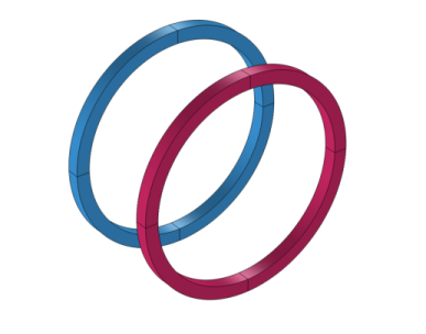
The geometry is now complete. To see its interior, click the Wireframe Rendering button in the Graphics toolbar.
 |
|
1
|
|
2
|
|
3
|
In the tree, select Built-in>Air.
|
|
4
|
|
5
|
|
1
|
In the Model Builder window, under Component 1 (comp1) right-click Materials and choose Blank Material.
|
|
2
|
|
4
|
|
1
|
In the Model Builder window, under Component 1 (comp1) right-click Magnetic Fields (mf) and choose the domain setting Coil.
|
|
3
|
|
4
|
|
5
|
|
6
|
|
1
|
|
2
|
|
3
|
|
1
|
|
3
|
|
4
|
|
5
|
|
6
|
|
1
|
|
2
|
|
3
|
|
1
|
|
2
|
|
3
|
|
1
|
|
2
|
|
3
|
|
5
|
|
6
|
|
8
|
|
1
|
|
2
|
|
3
|
|
4
|
|
1
|
|
3
|
|
4
|
|
5
|
|
6
|
|
7
|
Click OK.
|
|
1
|
|
2
|
|
3
|
|
4
|
|
1
|
|
2
|
|
1
|
|
2
|
|
3
|
|
4
|
|
5
|
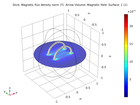
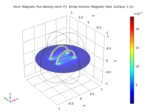
Click Replace Expression in the upper-right corner of the Expression section. From the menu, choose Component 1>Magnetic Fields>Magnetic>mf.normB - Magnetic flux density norm - T.
|
|
6
|
|
1
|
|
2
|
In the Settings window for Arrow Volume, click Replace Expression in the upper-right corner of the Expression section. From the menu, choose Component 1>Magnetic Fields>Magnetic>mf.Hx,mf.Hy,mf.Hz - Magnetic field.
|
|
3
|
Locate the Arrow Positioning section. Find the X grid points subsection. In the Points text field, type 24.
|
|
4
|
|
5
|
|
6
|
|
8
|
|
1
|
|
2
|
|
3
|
|
4
|
|
5
|
|
1
|
|
2
|
|
1
|
|
3
|
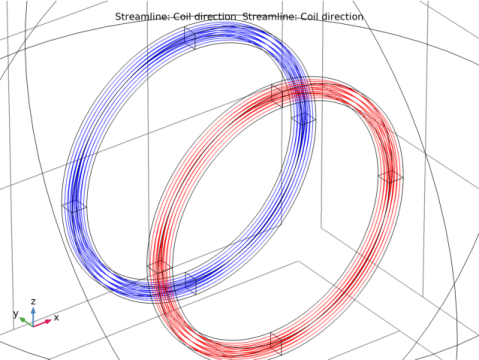
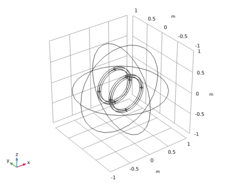
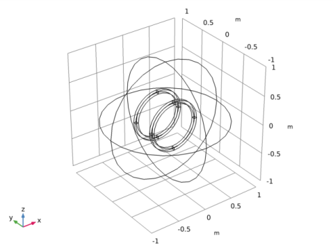
In the Settings window for Streamline, click Replace Expression in the upper-right corner of the Expression section. From the menu, choose Component 1>Magnetic Fields>Coil parameters>mf.coil1.eCoilx,...,mf.coil1.eCoilz - Coil direction.
|
|
1
|
|
3
|
In the Settings window for Streamline, click Replace Expression in the upper-right corner of the Expression section. From the menu, choose Component 1>Magnetic Fields>Coil parameters>mf.coil2.eCoilx,...,mf.coil2.eCoilz - Coil direction.
|
|
4
|
Locate the Coloring and Style section. Find the Point style subsection. From the Color list, choose Blue.
|
|
5
|