PDF

Generator in 3D
Introduction
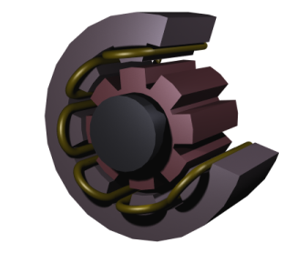
This example is a static 3D simulation of a generator comprising a rotor with permanent magnets. The center of the rotor consists of annealed medium carbon steel, which is a nonlinear ferromagnetic material which saturates at high magnetic flux density. The center is surrounded with several blocks of a permanent magnet made of samarium and cobalt, creating a strong magnetic field. The stator is made of the same nonlinear material as the center of the rotor, confining the field in closed loops through the winding. The winding (not included in the model) is wound around the stator poles. Figure 1 shows the generator with part of the stator sliced in order to show the winding and the rotor.
Figure 1: Drawing of a generator showing how the rotor, stator, and stator winding are constructed.
Model Definition
This model solves for the magnetic scalar potential, Vm, based on the assumption that currents can be neglected, which holds true when the generator terminals are open. The equation for Vm becomes
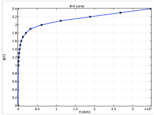
The stator and center of the rotor are made of annealed medium-carbon steel (soft iron), which is implemented in COMSOL Multiphysics as an interpolation function of the B-H curve of the material; see Figure 2.
Figure 2: The norm of the magnetic flux, |B|, versus the norm of the magnetic field, |H|, for the rotor and stator materials.
Results and Discussion
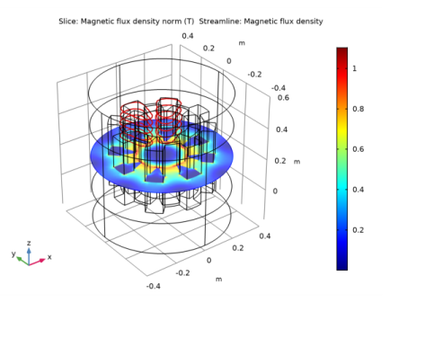
Figure 3 shows the norm of the magnetic flux for a slice through a centered cross section of the generator. The plot also shows the streamlines of the magnetic flux. The starting points of the streamlines have been carefully selected to show the closed loops between neighboring stator and rotor poles. A few streamlines are also plotted at the edge of the generator to illustrate the field there.
Figure 3: A combined slice and streamline plot of the magnetic flux density.
Application Library path: ACDC_Module/Motors_and_Actuators/generator_3d
Modeling Instructions
From the File menu, choose New.
New
In the New window, click Model Wizard.
Model Wizard
1
In the Model Wizard window, click 3D.
2
In the Select Physics tree, select AC/DC>Magnetic Fields, No Currents>Magnetic Fields, No Currents (mfnc).
3
Click Add.
4
Click Study.
5
In the Select Study tree, select General Studies>Stationary.
6
Click Done.
Geometry 1
Import 1 (imp1)
The geometry for this application is provided as a CAD file.
1
In the Home toolbar, click Import.
2
In the Settings window for Import, locate the Import section.
3
Click Browse.
4
5
Click Import.
6
Click the Wireframe Rendering button in the Graphics toolbar.
7
Click the Zoom Extents button in the Graphics toolbar.
Definitions
Cylindrical System 2 (sys2)
In the Definitions toolbar, click Coordinate Systems and choose Cylindrical System.
Add Material
1
In the Home toolbar, click Add Material to open the Add Material window.
2
Go to the Add Material window.
3
4
Click Add to Component in the window toolbar.
5
In the tree, select AC/DC>Soft Iron (Without Losses).
6
Click Add to Component in the window toolbar.
7
In the tree, select AC/DC>Hard Magnetic Materials>Sintered NdFeB Grades (Chinese Standard)>N50 (Sintered NdFeB).
8
Click Add to Component in the window toolbar.
9
In the Home toolbar, click Add Material to close the Add Material window.
Materials
Soft Iron (Without Losses) (mat2)
1
In the Model Builder window, under Component 1 (comp1)>Materials click Soft Iron (Without Losses) (mat2).
2
N50 (Sintered NdFeB) (mat3)
1
In the Model Builder window, click N50 (Sintered NdFeB) (mat3).
2
3
In the Settings window for Material, locate the Material Contents section.
4
5
In the Label text field, type Generic SmCo Magnet.
Magnetic Fields, No Currents (mfnc)
Magnetic Flux Conservation 2
1
In the Model Builder window, under Component 1 (comp1) right-click Magnetic Fields, No Currents (mfnc) and choose Magnetic Flux Conservation.
2
3
In the Settings window for Magnetic Flux Conservation, locate the Constitutive Relation B-H section.
4
From the Magnetization model list, choose B-H curve.
Magnetic Flux Conservation 3
1
In the Physics toolbar, click Domains and choose Magnetic Flux Conservation.
2
3
In the Settings window for Magnetic Flux Conservation, locate the Coordinate System Selection section.
4
From the Coordinate system list, choose Cylindrical System 2 (sys2).
5
Locate the Constitutive Relation B-H section. From the Magnetization model list, choose Remanent flux density.
6
Specify the e vector as
Magnetic Flux Conservation 4
1
In the Physics toolbar, click Domains and choose Magnetic Flux Conservation.
2
3
In the Settings window for Magnetic Flux Conservation, locate the Coordinate System Selection section.
4
From the Coordinate system list, choose Cylindrical System 2 (sys2).
5
Locate the Constitutive Relation B-H section. From the Magnetization model list, choose Remanent flux density.
Specify a reference level for the scalar magnetic potential by constraining the value at one point.
Zero Magnetic Scalar Potential 1
1
In the Physics toolbar, click Points and choose Zero Magnetic Scalar Potential.
2
The default Magnetic Insulation boundary condition applies in this case.
Mesh 1
1
In the Model Builder window, under Component 1 (comp1) click Mesh 1.
2
In the Settings window for Mesh, locate the Physics-Controlled Mesh section.
3
From the Element size list, choose Finer.
Free Tetrahedral 1
1
Right-click Component 1 (comp1)>Mesh 1 and choose Free Tetrahedral.
2
Click Build All.
Study 1
1
In the Model Builder window, click Study 1.
2
In the Settings window for Study, locate the Study Settings section.
3
Clear the Generate default plots check box.
4
In the Home toolbar, click Compute.
Results
3D Plot Group 1
In the Home toolbar, click Add Plot Group and choose 3D Plot Group.
Slice 1
1
Right-click 3D Plot Group 1 and choose Slice.
2
In the Settings window for Slice, locate the Plane Data section.
3
From the Plane list, choose XY-planes.
4
In the Planes text field, type 1.
5
Click Replace Expression in the upper-right corner of the Expression section. From the menu, choose Component 1>Magnetic Fields, No Currents>Magnetic>mfnc.normB - Magnetic flux density norm - T.
Streamline 1
1
In the Model Builder window, right-click 3D Plot Group 1 and choose Streamline.
2
3
In the Settings window for Streamline, locate the Coloring and Style section.
4
Find the Line style subsection. From the Type list, choose Tube.
5
In the 3D Plot Group 1 toolbar, click Plot.
6
Click the Zoom Extents button in the Graphics toolbar.