|
|
|
|
1
|
|
2
|
|
3
|
Click Add.
|
|
4
|
|
5
|
Click Add.
|
|
6
|
Click Study.
|
|
7
|
|
8
|
Click Done.
|
|
1
|
|
2
|
|
1
|
|
2
|
|
3
|
|
1
|
|
2
|
|
3
|
|
4
|
|
5
|
|
6
|
|
1
|
|
2
|
|
3
|
|
4
|
|
5
|
|
1
|
|
2
|
|
3
|
|
4
|
|
5
|
|
6
|
|
7
|
|
8
|
|
1
|
|
2
|
|
3
|
|
4
|
|
5
|
|
6
|
|
7
|
|
1
|
|
2
|
|
3
|
|
4
|
|
5
|
|
6
|
|
7
|
|
9
|
|
1
|
|
2
|
|
1
|
|
3
|
|
4
|
|
5
|
|
1
|
|
3
|
|
4
|
|
5
|
|
1
|
|
2
|
|
3
|
|
4
|
|
5
|
|
6
|
|
7
|
Click OK.
|
|
1
|
|
2
|
|
1
|
|
2
|
|
3
|
|
4
|
|
5
|
|
6
|
|
7
|
Click OK.
|
|
1
|
|
2
|
|
1
|
|
3
|
|
4
|
|
1
|
In the Model Builder window, under Component 1 (comp1)>Global ODEs and DAEs (ge) click Global Equations 1.
|
|
2
|
|
4
|
|
5
|
|
6
|
Click Filter.
|
|
7
|
|
8
|
Click OK.
|
|
9
|
|
10
|
|
11
|
|
12
|
Click Filter.
|
|
13
|
|
14
|
Click OK.
|
|
1
|
|
1
|
|
2
|
|
3
|
|
4
|
Locate the Constitutive Relation B-H section. From the Magnetization model list, choose Remanent flux density.
|
|
5
|
Specify the e vector as
|
|
1
|
|
2
|
|
3
|
|
4
|
|
1
|
|
1
|
|
2
|
|
3
|
In the tree, select Built-in>Air.
|
|
4
|
|
1
|
|
2
|
In the tree, select AC/DC>Copper.
|
|
3
|
|
4
|
In the tree, select AC/DC>Hard Magnetic Materials>Sintered NdFeB Grades (Chinese Standard)>N50 (Sintered NdFeB).
|
|
5
|
|
6
|
|
1
|
|
2
|
|
1
|
|
2
|
|
3
|
|
1
|
|
2
|
|
1
|
|
2
|
|
3
|
|
1
|
|
2
|
|
3
|
|
1
|
|
2
|
|
3
|
|
4
|
|
5
|
|
6
|
|
1
|
|
2
|
|
1
|
|
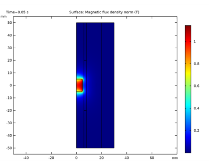
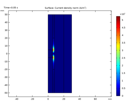
2
|
In the Settings window for Surface, click Replace Expression in the upper-right corner of the Expression section. From the menu, choose Model>Component 1>Magnetic Fields>Currents and charge>mf.normJ - Current density norm - A/m².
|
|
3
|
|
1
|
|
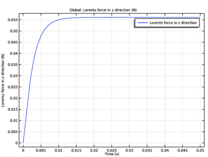
2
|
In the Settings window for Global, click Replace Expression in the upper-right corner of the y-axis data section. From the menu, choose Model>Component 1>Definitions>Variables>Fz - Lorentz force in z direction - N.
|
|
3
|
|
4
|
|
5
|
|
6
|
Click OK.
|
|
7
|
|
1
|
|
2
|
|
3
|
|
4
|
Click OK.
|
|
5
|
|
7
|
|
1
|
|
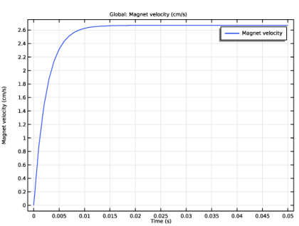
2
|
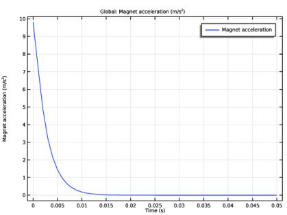
In the Settings window for Global, click Replace Expression in the upper-right corner of the y-axis data section. From the menu, choose Model>Component 1>Definitions>Variables>a - Magnet acceleration - m/s².
|
|
3
|
|
4
|
|
5
|
Click OK.
|
|
6
|