Prismatic Joint Theory

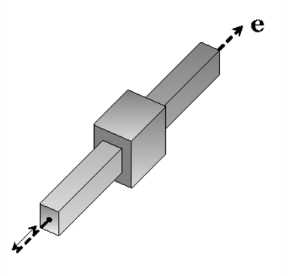
The Prismatic Joint, also known as a translational or sliding joint, has one translational degree of freedom between the two connected components. The components are free to translate, or slide, relative to each other along the joint axis.

The local coordinate system of a joint, which can be seen as rigidly connected to the source attachment, consists of three axes: joint axis (e1), second axis (e2), and third axis (e3). You specify the initial direction joint axis (e10), using one of the following methods:

	For all methods, the axis is normalized to give a unit vector.

In Method 3, the direction that has a positive projection on the global x-axis is selected. If the projection on the x-axis is very small (the edge is almost perpendicular to the x-axis), then the y-axis is used in the projection criterion. If the edge is perpendicular also to the y-axis, then the z-axis is used as the joint axis. You can also choose to reverse the direction of initial joint axis.

If the directions of the second and third axis are important (for example, when interpreting joint force results in the joint local coordinate system, or when there is elasticity in the joint), then Method 2 is preferred because this gives full control over all three axes. When an axis in the selected coordinate system is chosen to specify the joint axis, the other two axes are determined through cyclic permutation.

For Method 2 and Method 3, the initial second axis and initial third axis are computed internally as described below.

The initial second axis (e20) (perpendicular to the initial joint axis) is computed by making an auxiliary axis (eaux) (an axis not parallel to the initial joint axis) and then taking a cross product of the initial joint axis and this auxiliary axis:

The initial third axis (e30) is computed by taking a cross product of the initial joint axis and the initial second axis:

Finally, the rotated axes in the deformed configuration are formed by rotating the individual axes using the rotation matrix of the source attachment (Rsrc):

For 2D models, the generation of the coordinate system is significantly simplified. The initial third axis (e30) is taken as the out-of-plane axis (ez). The initial second axis (e20) is orthogonal to (e10) and (e30):

For a prismatic joint, the destination attachment is free to translate relative to the source attachment along the joint axis. The added degree of freedom is thus the relative displacement along the joint axis (u).

The translational motion of the source and destination attachments at the center of the joint can be computed as:

where, for the source and destination attachments, respectively:

•

uc,src and uc,dst are the displacement vectors for the attachments at the center of joint.

•

Rsrc and Rdst are the rotation matrices describing the rotation of each attachment.

To formulate this kind of connection for a rigid joint, the motion of the destination attachment is prescribed in terms of the motion of the source attachment:

The displacement vector (u) and quaternion vector (b) for the source and destination attachments are defined as:

The relative displacement vector in the global spatial coordinate system (ur) is defined as:

For 2D, the motion of the destination attachment is prescribed in terms of the motion of source attachment:

where φ is the rotation about z-axis (out-of-plane axis).

In the case that the joint is elastic, the elastic displacements and rotations are added to the source motion, so that the displacements and rotations at the center of joint is no longer equal for the source and destination attachments.

The elastic translation and rotation vectors are expressed in terms of the joint axes as

Here, u2, u3, θ1, θ2, and θ3 are the default elastic degrees of freedom available for this joint. Optionally, only a subset of them can be chosen to be elastic.