|
|
|
•
|
|
•
|
|
|
||
|
|
||
|
|
||
|
|
The scientific notation, such as 3.1416E-5, can be easier to read than decimal notation for tables containing values on different scales.
|
|
|
|
The engineering notation, such as 31.416E-6, is similar to scientific notation but with the powers of ten as multiples of three.
|
|
|
|
The decimal notation uses only decimal representation of the numbers, such as 0.000031416. Small numbers can get long representations because of leading zeros, and large numbers may appear with excess precision.
|
|
|
|
Display complex-valued numbers as the real part + the imaginary part followed by i (the imaginary unit), such as 2.451+0.657i.
|
|
|
|
||
|
|
||
|
|
||
|
|
||
|
|
For tables with filled data, click to plot the table as a Table Surface plot in the Graphics window.
|
|
|
|
||
|
|
Click to export the table to a text file in a spreadsheet format or to a Microsoft Excel Workbook (*.xlsx) if the license includes LiveLink™ for Excel®. When saving to a Microsoft Excel Workbook, an Excel Save dialog box opens where you can specify the sheet and range and whether to overwrite existing data and include a header.
|
|
|
|
||
|
|
||
|
|
||
|
|
||
|
|
||
|
|
||
|
|
||
|
|
||
|
|
|
|
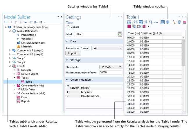
For a surface integration example that includes tables, see Effective Diffusivity in Porous Materials: Application Library path COMSOL_Multiphysics/Diffusion/effective_diffusivity.
|
|
|