Entering Quality Settings for Plot Settings Windows

Many plots have a section where you can select a plot resolution, enforce continuity, and specify the use of accurate derivative recovery. The steps for this section vary slightly based on the plot but are basically as follows.

Under , select a plot : , , , , , or . A higher resolution means that elements are split into smaller patches during rendering. The , , , use heuristics to determine a suitable resolution. For , enter a positive integer (default: 1) in the field. A higher value means higher resolution. The refinements is done by subdividing the element edges. See the following figure, which shows the refinement levels 1, 2, and 3:

Figure 21-1: Element refinement levels 1 (left), 2 (middle), and 3 (right).

For new plots, you can also specify a preference for the resolution on the page in the dialog box.


	Custom refinement applies to the base dataset. The number of elements in the model can therefore increase radically if the plot uses, for example, a revolve dataset, since the refinement is applied to the solution dataset.

To enforce continuity on discontinuous data, under , from the list, select:

: to plot elements independently.

(the default): to smooth the quantity within domains shared by the same material but not across material boundaries. Here, material is interpreted in a wider sense than just a physical material. Some physics interfaces implement material groups, which are sets of domains that are considered as being suitable for internal smoothing.

: to smooth the quantity inside the geometry, but no smoothing takes place across borders between domains with different settings.

: to apply smoothing to the entire geometry.

: to use an expression to indicate where smoothing should occur. Enter an expression in the field such that smoothing occurs where the expression is continuous. The default expression is dom, the domain variable, which is equivalent to the smoothing. You can also — in a surface plot, for example — use material.domain, which is an indicator variable for domains that share the same material (see Material Group Indicator Variables) and is equivalent to the setting.

The smoothing is done so that if there are two different values in points with the same coordinates, the plotted value is the mean of those two values.

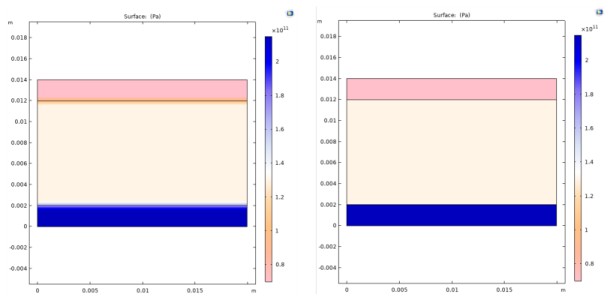
The default, , is to smooth the quantity except across borders between domains with different materials, where there is often a sharp transition from one material to another or between different types of physics. See the screenshots below that shows a material discontinuity where smoothing everywhere blurs the border (left) whereas smoothing inside material domains (right) keeps the material discontinuity intact. In these plots, no refinement is used to show the smoothing effect more clearly.

Figure 21-2: Smoothing everywhere (left) versus smoothing inside material domains (right).

Under , the default is because the accurate derivative recovery takes processing time. This recovery is a polynomial-preserving recovery that recovers fields with derivatives such as stresses or fluxes with a higher theoretical convergence than smoothing (see Polynomial-Preserving Derivative Recovery).

To use accurate derivative recovery, from the list, select:

: to perform recovery inside domains.

: to apply recovery to all domain boundaries.


	The Recover option only affects variables that are defined on domains.

Polynomial-Preserving Derivative Recovery

Plotting and evaluating stresses or fluxes boils down to evaluating space derivatives of the dependent variables. By default, computing a derivative like ux or uxx (first and second derivatives of u with respect to x) is done by evaluating the derivative of the shape functions used in the finite element approximation. These values have poorer accuracy than the solution u itself. For example, uxx is identically 0 if u is defined using linear elements. COMSOL Multiphysics evaluates the derivatives (and u itself) using a polynomial-preserving recovery technique by Z. Zhang (see Ref. 1). The recovery is only applied on variables that are discretized using Lagrange shape functions.

The polynomial-preserving recovery is a variant of the superconvergent patch recovery by Zienkiewicz and Zhu that forms a higher-order approximation of the solution on a patch of mesh elements around each mesh vertex. For regular meshes, the convergence rate of the recovered gradient is O(hp+1) — the same as for the solution itself. Near boundaries, the accuracy is not as good, and it might even be worse than without recovery. Results evaluation is about 2–5 times slower when using polynomial-preserving derivative recovery.

By default, the accurate derivative recovery smooths the derivatives within each group of domains with equal settings. Thus, there is no smoothing across material discontinuities. You find the setting for accurate derivative recovery in the plot node’s windows’ section. Due to performance reasons, the default value for list is (that is, no accurate derivative recovery). Select to smooth the derivatives within each domain group (that is, groups of domains with equal settings). Select to smooth the derivatives across the entire geometry.

Reference

1. A. Naga and Z. Zhang, “The Polynomial-Preserving Recovery for Higher Order Finite Element Methods in 2D and 3D”, Discrete and Continuous Dynamical Systems — Series B, vol. 5, pp. 769–798, 2005.