Turbulence Modeling

Turbulence is a property of the flow field and it is characterized by a wide range of flow scales: the largest occurring scales, which depend on the geometry, the smallest, quickly fluctuating scales, and all the scales in between. The propensity for an isothermal flow to become turbulent is measured by the Reynolds number

where μ is the dynamic viscosity, ρ the density, and U and L are velocity and length scales of the flow, respectively. Flows with high Reynolds numbers tend to become turbulent. Most engineering applications belong to this category of flows.

The Navier-Stokes equations can be used for turbulent flow simulations, although this would require a large number of elements in order to capture the wide range of scales in the flow. An alternative approach is to divide the flow quantities into mean values and fluctuations. When solving for the mean-flow quantities, the effect of the fluctuations is modeled using a turbulence closure. The idea behind this approach is that solving the model for the turbulence closure is numerically less expensive than resolving all the turbulence scales. Different turbulence closures invoke different assumptions on the modeled fluctuations, resulting in various degrees of accuracy for different flow cases.

This module includes turbulence models based on the Reynolds-averaged Navier-Stokes (RANS) model, which is the model type most commonly used in industrial flow applications.

The following assumes that the fluid is incompressible and Newtonian in which case the Navier-Stokes equations take the form:

Once the flow has become turbulent, all quantities fluctuate in time and space. It is seldom worth the extreme computational cost to obtain detailed information about the fluctuations. An averaged representation often provides sufficient information about the flow.

The Reynolds-averaged representation of turbulent flows divides the flow quantities into an averaged value and a fluctuating part,

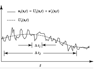
where

can represent any scalar quantity of the flow. In general, the mean value can vary in space and time. This is exemplified in Figure 4-6, which shows time averaging of one component of the velocity vector for nonstationary turbulence. The unfiltered flow has a time scale Δt1. After a time filter with width Δt2 >> Δt1 has been applied, there is a fluctuating part, u′i, and an average part, Ui. Because the flow field also varies on a time scale longer than Δt2, Ui is still time-dependent but is much smoother than the unfiltered velocity ui.

Decomposition of the flow field into an averaged part and a fluctuating part, followed by insertion into the Navier-Stokes equation, and averaging, gives the Reynolds-averaged Navier-Stokes (RANS) equations:

where U is the averaged velocity field and ⊗ is the outer vector product. A comparison with Equation 4-68 indicates that the only difference is the appearance of the last term on the left-hand side of Equation 4-69. This term represents the interaction between the fluctuating parts of the velocity field and is called the Reynolds stress tensor. This means that to obtain the mean flow characteristics, information about the small-scale structure of the flow is needed. In this case, that information is the correlation between fluctuations in all three directions.

The most common way to model turbulence is to assume that the turbulence is of a purely diffusive nature. The deviating part of the Reynolds stress is then expressed as

where μT is the eddy viscosity, also known as the turbulent viscosity. The spherical part can be written

where k is the turbulent kinetic energy. In simulations of incompressible flows, this term is included in the pressure, but when the absolute pressure level is of importance (in compressible flows, for example) this term must be explicitly included.

If the Reynolds average is applied to the compressible form of the Navier-Stokes equations, terms of the form

appear and need to be modeled. To avoid this, a density-based average, known as the Favre average, is introduced:

It follows from Equation 4-70 that

and a variable, ui, is decomposed into a mass-averaged component,

, and a fluctuating component, ui″, according to

Using Equation 4-71 and Equation 4-72 along with some modeling assumptions for compressible flows (Ref. 7), Equation 4-14 and Equation 4-15 can be written on the form

The Favre-averaged Reynolds stress tensor is modeled using the same argument as for incompressible flows:

where k is the turbulent kinetic energy. Comparing Equation 4-73 to its incompressible counterpart (Equation 4-69), it can be seen that except for the term

the compressible and incompressible formulations are exactly the same, except that the free variables are

instead of

More information about modeling turbulent compressible flows can be found in Ref. 1 and Ref. 7.

The turbulent transport equations are used in their fully compressible formulations (Ref. 8).