Several of the physics interfaces vary only by one or two default settings (see Table 4-1) in the Physical Model and Turbulence sections, which are selected either from a check box or drop-down list. For the Single-Phase Flow branch, all except the Rotating Machinery interfaces have the same Name (spf). The differences are based on the default settings required to model that type of flow as described in Table 4-1. 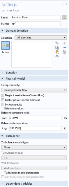Figure 4-1 shows the Settings window for Laminar Flow where you choose the type of compressibility (incompressible, weakly compressible or compressible at Mach numbers below 0.3) and the turbulence type and model (or none for laminar flow), and a check box to model Stokes flow by neglecting the inertial term.

The Creeping Flow Interface () models the Navier-Stokes equations without the contribution of the inertia term. This is often referred to as Stokes flow and is appropriate for flow at small Reynolds numbers, such as in very small channels or in microfluidic applications.

The Laminar Flow Interface () is used primarily to model flow at small to intermediate Reynolds numbers. The physics interface solves the Navier-Stokes equations, and by default assumes the flow to be incompressible; that is, the density is assumed to be constant.

You can also describe other material properties such as density by entering equations for its dependence on fluid composition and pressure (for compressible flow), or temperature. Many materials in the material libraries use temperature- and pressure-dependent property values. If the density is affected by temperature, a nonisothermal flow interface may be applicable (see The Nonisothermal Flow and Conjugate Heat Transfer, Laminar Flow, Turbulent Flow and LES Interfaces).

The various forms of the Single-Phase Flow, Turbulent Flow interfaces () model flow of large Reynolds numbers. The interfaces solve the Reynolds-averaged Navier-Stokes (RANS) equations for the filtered velocity field and filtered pressure as well as models for the turbulent viscosity. See The Creeping Flow, Laminar Flow, Turbulent Flow, and Large Eddy Simulation Interfaces for links to the physics interface information.

There are several turbulence models available: two algebraic turbulence models, the Algebraic yPlus and L-VEL models, and six transport-equation models, including a standard k-ε model, the Realizable k-ε model, a k-ω model, an SST model, a Low Reynolds number k-ε model, the Spalart-Allmaras model, and the v2-f model. Each model has its merits and weaknesses. See the Theory for the Turbulent Flow Interfaces for more details.

The Rotating Machinery, Laminar and Turbulent Flow Interfaces () model fluid flow in geometries with rotating parts. For example, stirred tanks, mixers, propellers and pumps.