Basics of Acoustics

Acoustics is the physics of sound. Sound is the sensation, as detected by the ear, of very small rapid changes in the acoustic pressure p above and below a static value p0. This static value is the atmospheric pressure (about 100,000 pascals).

The amplitude of the small pressure variations that can be detected by the human ear vary from roughly 2·10-5 Pa at the hearing threshold to 20 Pa for jet engine noise. The amplitude at normal speech levels is about 0.02 Pa. The amplitudes described here are often given on a the logarithmic decibel scale, relative to the hearing threshold value of 2·10-5 Pa, in units of dB SPL.

The acoustic pressure variations are typically described as pressure waves propagating in space and time. The wave crests are the pressure maxima while the troughs represent the pressure minima.

In more general terms, sound is created when the fluid is disturbed by a source. An example is a vibrating object, such as a speaker cone in a sound system. It is possible to see the movement of a bass speaker cone when it generates sound at a very low frequency. As the cone moves forward it compresses the air in front of it, causing an increase in air pressure. Then it moves back past its resting position and causes a reduction in air pressure. This process continues, radiating a wave of alternating high and low pressure at the speed of sound.

The frequency f (SI unit: Hz = 1/s) is the number of vibrations (pressure peaks) perceived per second and the wavelength λ (SI unit: m) is the distance between two such peaks. The speed of sound c (SI unit: m/s) is given as the product of the frequency and the wavelength, c = λf. It is often convenient to define the angular frequency ω (SI unit: rad/s) of the wave, which is ω = 2πf, and relates the frequency to a full 360o phase shift. The wave number k (SI unit: rad/m) is defined as k = 2π/λ. The wave number, which is the number of waves over a specific distance, is also usually defined as a vector k, such that it also contains information about the direction of propagation of the wave, with |k| = k. In general, the relation between the angular frequency ω and the wave number k is called the dispersion relation; for simple fluids it is ω/k = c.

The equations that describe the propagation of sound in fluids are derived from the governing equations of fluid flow. That is, conservation of mass, which is described by the continuity equation; the conservation of momentum, which is often referred to as the Navier-Stokes equations; an energy conservation equation; the constitutive equations of the model; and an equation of state to describe the relation between thermodynamic variables. In the classical case of pressure acoustics, which describes most acoustic phenomena accurately, the flow is assumed lossless and adiabatic, viscous effects are neglected, and a linearized isentropic equation of state is used.

Under these assumptions, the acoustic field is described by one variable, the pressure p (SI unit: Pa), and is governed by the wave equation

where t is time (SI unit: s), ρ0 is the density of the fluid (SI unit: kg/m3), and c is the (adiabatic) speed of sound (SI unit: m/s).

Acoustic problems often involve simple harmonic waves such as sinusoidal waves. More generally, any signal may be expanded into harmonic components via its Fourier series. The wave equation can then be solved in the frequency domain for one frequency at a time. A harmonic solution has the form

where the spatial p(x) and temporal sin(ωt) components are split. The pressure may be written in a more general way using complex variables

where the actual (instantaneous) physical value of the pressure is the real part of Equation 1. Using this assumption for the pressure field, the time-dependent wave equation reduces to the well-known Helmholtz equation

In the homogeneous case, one simple solution to the Helmholtz equation (Equation 2) is the plane wave

where P0 is the wave amplitude, and it is moving in the k direction with angular frequency ω and wave number k = |k|.

In most practical situations, an exact analytical solution to Equation 2 does not exist. Solving the equation requires a numerical approach using simulations.

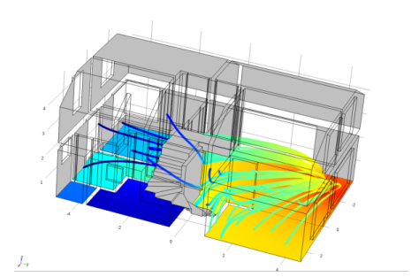
As mentioned, solving the governing equations for the acoustic problems analytically — like, for example, the Helmholtz equation (Equation 2) — is only possible in a few simple situations. In order to solve real-life industrial problems, which can very well be multiphysics problems involving several coupled physics, numerical methods are necessary. This is the job of COMSOL Multiphysics. In the Acoustics Module, most of the physics interfaces are based on the finite element method (FEM). In order to extend the range of models that can be solved, the Acoustics Module also includes the Pressure Acoustics, Boundary Elements interface based on BEM, two interfaces based on the discontinuous Galerkin (dG-FEM) method, and Ray Acoustics that uses a ray tracing method.

Solving a model using FEM requires a computational mesh. The solution is approximated on each mesh element (the finite elements) by a shape function (a local basis or interpolation function). Setting up this system of mesh elements and local shape functions leads to a discrete vector-matrix problem that needs to be solved. After solving the matrix problem with an adequate method, the solution to the original problem can be reconstructed. When solving wave problems numerically, one should be aware of the time and length scales involved in the problem, as will be discussed below.

When solving acoustic problems, it is important to think about the different basic length and time scales involved in the system. Some of the scales are set by the physics of the problem, while others are set by the numerical solution method. The relative size of these scales may influence the accuracy of the solution but also the selection of the physics interface used to model the problem.

When working with acoustics in the frequency domain, that is, solving the Helmholtz equation, only one time scale T exists (the period) and it is set by the frequency, T = 1/f. Several length scales exist: the wavelength λ = c/f, the smallest geometric dimension Lmin, the mesh size h, and the thickness of the acoustic boundary layer δ (the latter is discussed in Models with Losses). In order to get an accurate solution, the mesh should be fine enough to both resolve the geometric features and the wavelength. As a rule of thumb, the maximal mesh size should be less than or equal to λ/N, where N is a number between 5 and 10, and depends on the spatial discretization.

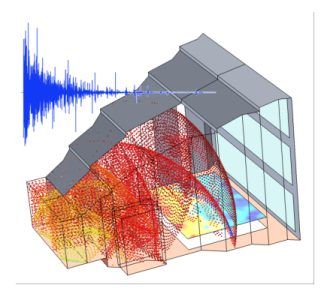
Note that when the wavelength becomes smaller than the characteristic length scale in the model, the two interfaces in Geometrical Acoustics can be used. The equations solved here do not require the same mesh constraints and can be used to model much larger systems (measured in wavelengths) compared to solving, for example, the Helmholtz equation.

For transient acoustic problems the same considerations apply. However, several new time scales are also introduced. One is given by the frequency contents of the signal and by the desired maximal frequency resolution: T = 1/ fmax. The other is given by the size of the time step Δt used by the numerical solver. A condition on the so-called CFL number dictates the relation between the time step size and the minimal mesh size hmin, The CFL number is defined as

where c is the speed of sound in the system. For all the transient interfaces available with the Acoustics Module the solver is automatically set up to meet the CFL criterion. The user is only required to enter the maximal frequency fmax to be resolved by the model.

In order to run accurate acoustic simulations, it is important to think about these physical and numerical scales and about their influence on the convergence and correctness of the numerical solution. A good practical approach is to test the robustness of a solution compared to changes in the mesh in all cases and the numerical time stepping in the transient problems. If some measure of the solution, within a given accuracy range, changes when the mesh is refined then the mesh was probably not good enough.

Boundary conditions define the nature of the boundaries of the computational domain. Some define real physical obstacles, like a sound hard wall or a moving interface. Others, called artificial boundary conditions, are used to truncate the domain. The artificial boundary conditions are, for example, used to simulate an open boundary where no sound is reflected. It may also mimic a reacting boundary such as a perforated plate.

The propagation of sound in solids happens through small-amplitude elastic oscillations of the solids shape and structure. These elastic waves are transmitted to surrounding fluids as ordinary sound waves. Through acoustic-structure interaction, the fluid pressure causes a fluid load on the solid domain, and the structural acceleration affects the fluid domain as a normal acceleration across the fluid-solid boundary.

The Acoustics Module has the Poroelastic Waves interface available to model poroelastic waves that propagate in porous materials. These waves result from the complex interaction between acoustic pressure variations in the saturating fluid and the elastic deformation of the solid porous matrix.

In order to accurately model acoustics in geometries with small dimensions, it is necessary to include thermal conduction effects and viscous losses explicitly in the governing equations. Near walls, viscosity and thermal conduction become important because the acoustic field creates viscous and thermal boundary layers where losses are significant. A detailed description is needed to model these phenomena; the dedicated Thermoviscous Acoustics, Frequency Domain interface solves the full linearized Navier-Stokes, continuity, and energy equations simultaneously. The physics interface solves for the acoustic pressure p, the particle velocity vector u, and the acoustic temperature variation T. These are the acoustic variations on top of the mean background values.

The length scale at which the thermoviscous acoustic description is necessary is given by the thickness of the viscous (v) and thermal (th) boundary layers

where μ is the dynamic viscosity, k is the coefficient of thermal conduction, and Cp is the specific heat capacity at constant pressure. These two length scales define an acoustic boundary layer that needs to be resolved by the computational mesh.

Another way to introduce losses in the governing equations is to use the equivalent fluid models available in the pressure acoustics interfaces. In a homogenized way, this introduces attenuation properties to the bulk fluid that mimic different loss mechanisms. This is in contrast to the thermoviscous acoustics interfaces that model losses explicitly where they happen, that is, in the acoustic boundary layer near walls. The fluid models include losses due to bulk thermal conduction and viscosity (in the main Pressure Acoustics domain feature), models for simulating the damping in certain porous materials (in the Poroacoustics domain feature), and models to mimic the boundary absorption losses in long narrow ducts (the Narrow Region Acoustics domain feature). When applicable, the equivalent fluid models are computationally much less heavy than, for example, solving a corresponding full poroelastic model.

At high frequencies when the wavelength is much smaller than the characteristic geometric features, it is impractical to solve acoustic problems using pressure acoustics. Here, other methods are used like, for example, ray methods or energy diffusion analogies. These are known as geometrical acoustics methods and are used for modeling room acoustics, concert hall acoustics, and outdoor propagation over large distances. The Geometrical Acoustics branch includes the Ray Acoustics and the Acoustic Diffusion Equation interfaces.