As this critical value is reached, cracks grow and spread until the material fractures. The occurrence and growth of the cracks play an important role in the failure of brittle materials. There are a number of theories to describe such behavior. In the continuum damage mechanics formalism, a damage variable represents the amount of deterioration due to crack growth. This damage variable controls the weakening of the material’s stiffness, and it produces a nonlinear relation between stress and strain.

For a linear elastic material, Hooke’s law relates the undamaged stress tensor σun to the elastic strain tensor:

here, is the fourth order elasticity tensor, “:” stands for the double-dot tensor product (or double contraction). The elastic strain εel is the difference between the total strain ε and all inelastic strains εinel. There may also be an extra stress contribution σex, with contributions from initial, external or viscoelastic stresses.

For the scalar damage models, the damaged stress tensor σd is computed from the undamaged stress as

This damaged stress is then used in weak formulation. There are different ways to compute the scalar damage variable d that controls the material weakening. These are listed in the following sections.

The strain-based formulation for the damage model is based on the loading function f such as

here, εeq is the equivalent strain, a scalar measure of the elastic strain; and κ is a state variable. The evolution of the state variable κ follows the Kuhn-Tucker loading/unloading conditions

In this formulation, κ is the maximum value of εeq in the load history. The damage variable d is then computed as a function of the state variable κ and other parameters.

Different damage models use different definitions for the equivalent strain εeq. The Rankine damage model defines the equivalent strain from the largest undamaged principal stress σp1 as

here, the symbol “<>” are the Macaulay brackets, and E is Young’s modulus. The Macaulay brackets are used since in this formulation only tensile (positive) stresses cause damage.

The Smooth Rankine damage model defines the equivalent strain from the three undamaged principal stresses

In both the Rankine and the Smooth Rankine damage models, by default only the principal stresses in tension contribute to the damage evolution, but it is also possible to activate damage in compression by including the compressive stresses in the computation of the damaged stress tensor σd.

The Euclidean Norm of the elastic strain tensor can also be used as a measure for the equivalent strain

For Mazars damage for concrete, it is also possible to select from Mazars or Modified Mazars equivalent strain. For Mazars equivalent strain is defined as

In the Modified Mazars equivalent strain (Ref. 2 and Ref. 3), a correction factor γ is added to improve the approximation of the failure surface of concrete in multiaxial compression.

It is also possible to apply a User defined expression for defining the equivalent strain as a function of undamaged stress, stress components or strains.

A key component in a scalar damage model is the definition of the damage evolution law. The Linear strain softening law defines the damage variable from

Here, ε0 denotes the onset of damage, computed from the tensile strength σts and Young’s modulus E, so that ε0 = σts/E. The parameter εf is derived from parameters such as the tensile strength, the characteristic element size hcb and the fracture energy per unit area Gf, or the fracture energy per unit volume gf.

The Exponential strain softening law defines the damage evolution from

The Mazars damage for concrete utilizes two different damage evolution laws, one for tensile damage and another for compressive damage. These two damage functions are combined as

here, αt and αc are weight functions depending on the current stress state, and β determines the response in shear, i.e. the evolution of the combined damage function in states where both damage functions are active.

To define the tensile damage evolution law dt(κ) (Ref. 3), it is possible to use either Linear strain softening, Exponential strain softening, or the Mazars damage evolution function, which is obtained by a combination of linear and exponential strain softening

Here, At and Bt are tensile damage evolution parameters, and ε0t is the tensile strain threshold.

The compressive damage evolution law dc(κ) is obtained by the Mazars damage evolution function

Here, Ac and Bc are compressive damage evolution parameters, and ε0c is the compressive strain threshold. Both the tensile and compressive damage evolution laws can also be specified by User defined expressions.

The most common application for the damage models is to describe strain localization, due to for example cracking in quasi-brittle materials. In a damage model without regularization, the deformation during strain softening will always localize in the narrowest possible band, following the principle of least action. This means that large strains will develop in a narrow band of elements (or even Gauss points). As a consequence, the amount of dissipated energy during softening will decrease upon mesh refinement. The results of a damage model without regularization will therefore be mesh dependent and possibly unstable, hence there is the need for these models to be regularized for the solution to maintain its mesh objectivity.

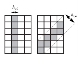
This simplest regularization technique is based on stress-strain curves (damage evolution laws) that depend on the mesh and element characteristics. The method is often called the Crack Band method (Ref. 4, Ref. 5). The method regularizes the solution from a global viewpoint, which dissipates the correct amount of energy during strain localization. The main difficulty in using the crack band method is to find the correct width of the crack band, hcb, which can depend on the element size and shape as well as the order of the interpolation and the current stress state (i.e. inclination of the crack with respect to the mesh).

The length scale used in the crack band method is computed by using the volume to area ratio in the mesh elements. By using the element volume v in 3D or the area a in 2D, the crack band width hcb is defined as:

The crack band width hcb is then used to modify the Damage evolution law in which the damage variable d(κ) is computed. Note that the damage evolution laws (Equation 3-73 and Equation 3-74) are unaffected by the crack band method.

The Implicit Gradient method (Ref. 6) enforces a predefined width of the damage zone through a localization limiter. This is achieved by adding a nonlocal strain variable, the nonlocal equivalent strain εnl, through an additional PDE where the equivalent strain εeq acts as source term. This PDE is solved simultaneously with the displacement field:

Here, the parameter c controls the width of the localization band. This parameter is defined from the Internal length scale lint, and the geometry dimension n (two or three dimension)

If the fracture energy per unit area is used to define the softening behavior, the size of the damage zone also needs to be entered as an input. This is not necessarily the same as lint.

The strain-based formulation for the damage model (Equation 3-62) is then redefined by the nonlocal equivalent strain εnl instead of the equivalent strain εeq