Stress Linearization
Stress linearization is a procedure in which the stress distribution along a line through the thickness in a solid is approximated with an equivalent linear stress distribution, similar to what would be the result of an analysis using shell theory. The line is commonly referred to a stress classification line, SCL. This type of evaluation is common is the analysis of pressure vessels. It is also useful for the dimensioning of reinforcements for concrete structures, and for fatigue analysis of welds.
To perform a stress linearization, you add one Stress Linearization node for each SCL.
Orientation of Stress Components
The stresses along the SCL are represented in a local orthonormal coordinate system, x1-x2-x3. The x1 direction is oriented along the SCL, so it is mainly the stresses in the second and third directions which are of interest.
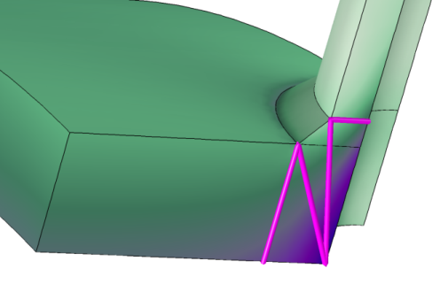
In 3D, you must specify the x2 direction, and thus implicitly the x3 direction. You specify the orientation either by selecting a point in the x1-x2 plane, or by defining an orientation vector in an approximate x2 direction. In either case, the actual x2 direction is chosen so that it is perpendicular to the SCL, and lies in the plane you have specified. The x3 orientation is then taken as perpendicular to x1 and x2. As long as you are only interested in a stress intensity, the choice of orientation is arbitrary.
In 2D, the x3 direction is the out-of-plane direction, and the x2 direction is perpendicular to the SCL in the X-Y plane.
In 2D axial symmetry, the x3 direction is the azimuthal direction, and the x2 direction is perpendicular to the SCL in the R-Z plane.
Creating the Stress Classification Line
The most straightforward way to create an SCL, is to include it in the geometry, and then select it in a Stress Linearization node.
Figure 2-22: Four stress classification lines in a transition region at a pressure vessel nozzle.
There are, however, some situations where the direct approach is less convenient:
In this case, a possible solution is to operate on a copy of the geometry in another component. It is then possible to use submodeling — that is, to study only a local region with its boundaries having displacements controlled by the solution from the larger model.
Below is an outline of the steps you need to take for this approach.
1
In the original component (assume that its tag is comp1), add a General Extrusion operator. Set Source frame to Material. You can name the operator, but in the following description, the default name genext1 is assumed. This operator will be used for mapping results to the second component.
2
3
Add the geometry, using for example Insert Sequence or Import. to the new component (comp2).
4
5
6
Add a Prescribed Displacement node having domain selection. Select All domains. Prescribe the displacement in all directions to be the same as in the original model with expressions like comp1.genext1(u) for Prescribed in x direction.
7
If the original analysis contains inelastic strains, such as thermal expansions, these must also be included. You can do this either by adding a Thermal Expansion node with appropriate settings, or by explicitly importing the inelastic strains using an External Strain node. In the latter case, you would use expressions like comp1.genext1(solid.eth11) for the strain components.
8
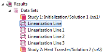
Add Stress Linearization nodes for the new linearization lines.
9
Add the materials that were used in comp1. The most efficient approach is to add them under Global Definitions, and link to the same material definitions from both components.
10
Create a mesh for the domains in comp2 which you are solving for. It is only the mesh close to the new edges to which you need to pay any attention.
11
12
In the settings for the new study set Values of variables not solved for to point to the solution from which you want to pick the results in comp1. You can also add an Auxiliary sweep, if the original analysis contains results for several parameters or time steps.
13
Studies and Solutions
Stress linearization is a pure postprocessing operation. The Stress Linearization node will only create a number of variables, which can be evaluated under Results. It is thus possible to add such nodes after the main analysis has been performed. In order to make the new variables available for postprocessing, you must then run an Update Solution.
Results
When you have included one or more Stress Linearization nodes in a model, a number of data sets and an extra default plot are generated.
One edge data set is created for each SCL. These data sets are named Linearization Line <n>, where n is an integer number.
Figure 2-23: Generated data sets in a model with four SCL.
The default plot contains graphs for the 22 component of the actual stress, the membrane stress, and the linearized stress. The first Linearization Line data set is selected. By changing edge date set in the plot group, you can easily move between the different stress classification lines.
Figure 2-24: Default plot along a stress classification line.
Variable Names
Each Stress Linearization node adds a number of variables. Many of these variables exist with two different scopes, physics scope and feature scope. The physics scope is the name of the physics interface, having the default value ‘solid’. The feature scope contains also the tag of the Stress Linearization node, for example ‘sl1’.
As an example, the variable solid.Sm22 and the variable solid.sl1.Sm22 have the same value. The variables with physics scope makes it more convenient to create expressions using postprocessing. You could for example make a line plot of solid.sb22, and get all edges having a stress linearization colored by their individual results.
Sllij
ij = 11, 12, 13, 22, 23, 33
Smij
ij = 11, 12, 13, 22, 23, 33
Sbij
ij = 11, 12, 13, 22, 23, 33
Smbij
ij = 11, 12, 13, 22, 23, 33
Spsij
ij = 11, 12, 13, 22, 23, 33
Speij
ij = 11, 12, 13, 22, 23, 33
Nij
ij = 22, 23, 33
Mij
ij = 22, 23, 33
Qi
i = 2, 3
 
Stress Linearization in the Structural Mechanics Theory Chapter.