|
|
|


|
1
|
|
2
|
|
3
|
Click Add.
|
|
4
|
Click Study.
|
|
5
|
|
6
|
Click Done.
|
|
1
|
|
2
|
|
3
|
|
4
|
Click Browse.
|
|
5
|
Browse to the model’s Application Libraries folder and double-click the file effective_diffusivity.mphbin.
|
|
6
|
Click Import.
|
|
1
|
|
2
|
|
1
|
|
2
|
|
1
|
|
2
|
|
3
|
|
4
|
Click OK.
|
|
5
|
|
6
|
|
1
|
|
2
|
|
3
|
|
4
|
Click OK.
|
|
5
|
|
6
|
|
1
|
|
2
|
|
3
|
|
4
|
Click OK.
|
|
5
|
|
6
|
|
1
|
|
2
|
Clear the Convection check box.
|
|
1
|
In the Model Builder window, under Component 1 (comp1)>Transport of Diluted Species (tds) click Transport Properties 1.
|
|
2
|
|
3
|
|
1
|
In the Model Builder window, under Component 1 (comp1)>Transport of Diluted Species (tds) click Initial Values 1.
|
|
2
|
|
3
|
|
1
|
|
2
|
|
3
|
|
4
|
|
5
|
|
1
|
|
2
|
|
3
|
|
4
|
|
5
|
|
6
|
|
1
|
|
2
|
|
3
|
|
4
|
|
1
|
|
2
|
|
1
|
|
2
|
|
3
|
|
4
|
|
5
|
|
1
|
|
2
|
|
3
|
|
4
|
|
5
|
|
1
|
|
2
|
|
3
|
|
4
|
|
5
|
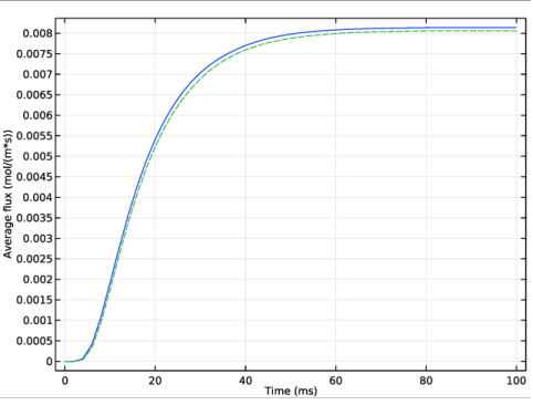
Click Replace Expression in the upper-right corner of the y-axis data section. From the menu, choose Component 1>Definitions>Variables>flux_avg - Average flux - mol/(m²·s).
|
|
1
|
|
2
|
|
3
|
|
4
|
|
5
|
|
6
|
In the associated text field, type Average flux (mol/(m*s)).
|
|
7
|
|
1
|
|
2
|
|
3
|
|
4
|
Locate the Expressions section. In the table, enter the following settings:
|
|
5
|
Click Evaluate.
|
|
1
|
Go to the Table window.
|
|
1
|
|
2
|
|
3
|
|
4
|
Find the Physics interfaces in study subsection. In the table, clear the Solve check box for Study 1.
|
|
5
|
|
6
|
|
1
|
|
2
|
|
3
|
Find the Physics interfaces in study subsection. In the table, clear the Solve check box for the Transport of Diluted Species (tds) interface.
|
|
4
|
|
5
|
|
6
|
|
1
|
|
2
|
|
4
|
|
5
|
|
1
|
|
2
|
|
1
|
|
2
|
|
3
|
Clear the Convection check box.
|
|
1
|
In the Model Builder window, under Component 2 (comp2)>Transport of Diluted Species 2 (tds2) click Transport Properties 1.
|
|
2
|
|
3
|
|
1
|
In the Model Builder window, under Component 2 (comp2)>Transport of Diluted Species 2 (tds2) click Initial Values 1.
|
|
2
|
|
3
|
|
1
|
|
3
|
|
4
|
|
5
|
|
1
|
|
3
|
|
4
|
|
5
|
|
6
|
|
1
|
|
2
|
|
1
|
|
2
|
|
3
|
|
4
|
|
1
|
|
2
|
|
3
|
|
4
|
|
5
|
|
1
|
|
2
|
|
3
|
|
5
|
Click Replace Expression in the upper-right corner of the y-axis data section. From the menu, choose Component 2>Definitions>Variables>flux_hom - Flux, 1D model - mol/(m²·s).
|
|
6
|
Click to expand the Coloring and Style section. Find the Line style subsection. From the Line list, choose Dashed.
|
|
7
|
|
1
|
|
2
|
|
3
|
|
1
|
|
2
|
|
3
|
|
4
|
|
1
|
|
2
|
|
3
|
|
4
|
|
5
|
|
6
|
Locate the Selections of Resulting Entities section. Select the Resulting objects selection check box.
|
|
7
|
|
1
|
|
2
|
|
3
|
|
4
|
|
1
|
|
2
|
|
3
|
|
4
|
|
5
|
|
6
|
|
7
|
|
1
|
|
2
|
|
3
|
|
4
|
|
5
|
|
6
|
Locate the Selections of Resulting Entities section. Select the Resulting objects selection check box.
|
|
7
|
|
1
|
|
2
|
|
3
|
|
4
|
|
5
|
Locate the Selections of Resulting Entities section. Select the Resulting objects selection check box.
|
|
6
|
|
1
|
|
2
|
Select the object fil1 only.
|
|
3
|
|
4
|
|
5
|
|
6
|
Locate the Selections of Resulting Entities section. Select the Resulting objects selection check box.
|
|
7
|
|
1
|
|
2
|
|
3
|
|
4
|
|
5
|
|
6
|
Locate the Selections of Resulting Entities section. Select the Resulting objects selection check box.
|
|
7
|
|
1
|
|
2
|
Select the object r1 only.
|
|
3
|
|
4
|
|
1
|
|
2
|
Select the object r2 only.
|
|
3
|
|
4
|
|
5
|
|
1
|
|
2
|
Select the object dif2 only.
|
|
3
|
|
4
|
|
1
|
|
2
|
Click in the Graphics window and then press Ctrl+A to select both objects.
|
|
3
|
|
4
|
|
5
|
|
6
|
|
7
|
|
1
|
|
2
|
|
3
|
|
4
|
|
1
|
|
2
|
On the object uni1, select Domain 1 only.
|
|
3
|
|
4
|
|
5
|
On the object uni1, select Boundaries 2 and 3 only.
|
|
1
|
|
2
|
|
3
|
|
4
|
|
5
|
On the object pard1, select Domains 2–9 only.
|
|
1
|
|
2
|
|
3
|
|
4
|
On the object fin, select Point 546 only.
|
|
5
|
|
6
|
|
1
|
|
2
|
|
3
|
|
4
|
On the object fin, select Boundary 1 only.
|
|
1
|
|
2
|
|
3
|
|
4
|
On the object fin, select Boundary 290 only.
|
|
5
|