|
|
|

|
1
|
|
2
|
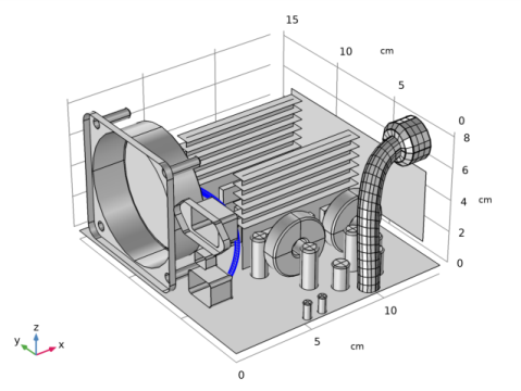
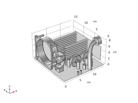
Browse to the model’s Application Libraries folder and double-click the file electronic_enclosure_cooling_geom.mph.
 |
|
1
|
|
2
|
|
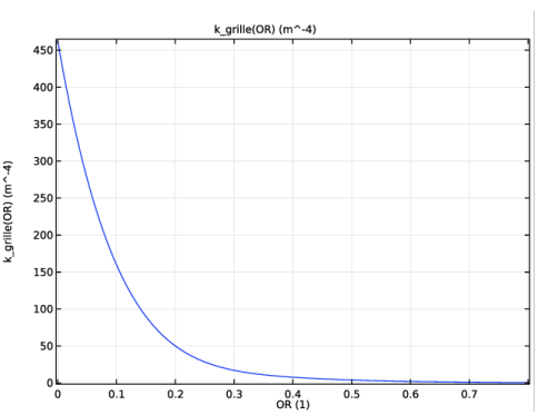
3
|
Locate the Definition section. In the Expression text field, type 12084*OR^6-42281*OR^5+60989*OR^4-46559*OR^3+19963*OR^2-4618.5*OR+462.89.
|
|
4
|
|
5
|
|
6
|
|
7
|
|
8
|
Click Plot.
|
|
1
|
|
2
|
|
3
|
In the tree, select Built-In>Air.
|
|
4
|
|
5
|
|
6
|
|
7
|
|
8
|
|
9
|
In the tree, select Built-In>Aluminum.
|
|
10
|
|
11
|
In the tree, select Built-In>Copper.
|
|
12
|
|
13
|
In the tree, select Built-In>Silicon.
|
|
14
|
|
15
|
|
1
|
|
2
|
|
1
|
|
2
|
|
3
|
|
1
|
|
2
|
|
3
|
|
1
|
|
2
|
|
3
|
|
1
|
|
2
|
|
3
|
|
1
|
|
2
|
|
3
|
|
1
|
In the Model Builder window, under Component 1 (comp1) right-click Materials and choose Layers>Single Layer Material.
|
|
2
|
|
3
|
|
4
|
|
5
|
|
1
|
|
2
|
|
3
|
Click OK.
|
|
1
|
|
2
|
|
3
|
|
4
|
|
5
|
|
1
|
|
2
|
In the tree, select Built-In>Copper.
|
|
3
|
Click OK.
|
|
1
|
|
2
|
|
3
|
|
4
|
|
5
|
|
1
|
|
2
|
|
3
|
|
1
|
|
2
|
|
3
|
Click to expand the Material Properties section. In the Material properties tree, select Basic Properties>Heat Capacity at Constant Pressure.
|
|
4
|
|
5
|
|
6
|
|
7
|
|
8
|
|
9
|
|
10
|
|
11
|
|
12
|
In the Diagonal table, enter the following settings:
|
|
13
|
click OK.
|
|
1
|
|
2
|
|
3
|
|
1
|
In the Model Builder window, under Component 1 (comp1)>Heat Transfer in Solids and Fluids (ht) click Fluid 1.
|
|
2
|
|
3
|
|
1
|
In the Model Builder window, under Component 1 (comp1)>Heat Transfer in Solids and Fluids (ht) click Initial Values 1.
|
|
2
|
|
3
|
|
1
|
|
2
|
|
3
|
|
4
|
|
5
|
|
1
|
|
2
|
In the Settings window for Heat Source, type Heat Source 2: Large Transformer Coil in the Label text field.
|
|
3
|
|
4
|
|
5
|
|
1
|
|
2
|
In the Settings window for Heat Source, type Heat Source 3: Small Transformer Coils in the Label text field.
|
|
3
|
|
4
|
|
5
|
|
1
|
|
2
|
|
3
|
|
4
|
|
5
|
|
1
|
|
2
|
In the Settings window for Heat Source, type Heat Source 5: Large Capacitors in the Label text field.
|
|
3
|
|
4
|
|
5
|
|
1
|
|
2
|
In the Settings window for Heat Source, type Heat Source 6: Medium Capacitors in the Label text field.
|
|
3
|
|
4
|
|
5
|
|
1
|
|
2
|
In the Settings window for Heat Source, type Heat Source 7: Small Capacitors in the Label text field.
|
|
3
|
|
4
|
|
5
|
|
1
|
|
2
|
|
3
|
|
4
|
|
1
|
|
2
|
|
3
|
|
4
|
|
1
|
|
2
|
|
3
|
|
1
|
|
2
|
|
3
|
|
4
|
|
1
|
|
2
|
|
3
|
|
1
|
|
2
|
|
3
|
|
4
|
|
5
|
Locate the Parameters section. From the Static pressure curve list, choose Static pressure curve data.
|
|
6
|
|
7
|
Browse to the model’s Application Libraries folder and double-click the file electronic_enclosure_cooling_fan_curve.txt.
|
|
8
|
Locate the Static Pressure Curve Interpolation section. From the Interpolation function type list, choose Piecewise cubic.
|
|
1
|
|
2
|
|
3
|
|
4
|
|
1
|
In the Model Builder window, under Component 1 (comp1)>Turbulent Flow, Algebraic yPlus (spf) click Initial Values 1.
|
|
2
|
|
3
|
Specify the u vector as
|
|
1
|
|
2
|
|
3
|
|
1
|
|
2
|
|
3
|
|
4
|
Click to expand the Advanced Settings section. In order to get a regular mesh, select the option to adjust the mesh position on the edges in the swept direction.
|
|
5
|
|
1
|
|
2
|
|
3
|
|
4
|
Click the Custom button.
|
|
5
|
|
7
|
|
9
|
|
1
|
|
2
|
|
3
|
|
4
|
|
1
|
|
2
|
|
3
|
|
4
|
|
5
|
Click the Custom button.
|
|
6
|
|
8
|
|
1
|
|
2
|
|
3
|
|
1
|
|
2
|
|
3
|
Click the Custom button.
|
|
4
|
|
6
|
|
8
|
|
10
|
|
12
|
|
14
|
|
1
|
|
2
|
|
3
|
|
1
|
|
2
|
|
3
|
|
4
|
|
1
|
|
2
|
|
3
|
|
4
|
|
5
|
|
6
|
Click to expand the Corner Settings section. From the Handling of sharp edges list, choose Trimming.
|
|
1
|
In the Model Builder window, expand the Boundary Layers 1 node, then click Boundary Layer Properties 1.
|
|
2
|
|
3
|
|
4
|
|
5
|
|
6
|
|
1
|
|
2
|
|
3
|
|
1
|
|
2
|
|
3
|
|
1
|
|
2
|
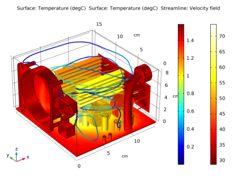
In the Settings window for Streamline, click Replace Expression in the upper-right corner of the Expression section. From the menu, choose Model>Component 1>Turbulent Flow, Algebraic yPlus>Velocity and pressure>u,v,w - Velocity field.
|
|
3
|
|
4
|
Locate the Coloring and Style section. Find the Line style subsection. From the Type list, choose Tube.
|
|
1
|
|
2
|
In the Settings window for Color Expression, click Replace Expression in the upper-right corner of the Expression section. From the menu, choose Model>Component 1>Turbulent Flow, Algebraic yPlus>Velocity and pressure>spf.U - Velocity magnitude - m/s.
|
|
3
|