Defining a Layered Material
Start by adding a Layered Material at the Materials node under Global Definitions. Then, take the following steps to define the laminate:
Add the required number of layers in the Layer Definition section of a Layered Material node.
Define the referenced materials under the Materials node. You can either add a Blank Material and fill in the required material properties or choose a material from the Material Library.
Note that required material properties for the material in a certain layer depends on the Solid Model chosen in the Linear Elastic Material node in Layered Shell or Layered Linear Elastic Material node in Shell interface.
For the Isotropic model (with Young’s modulus and Poisson’s ratio option), scalar values of Young’s modulus and Poisson’s ratio are required.
For the Orthotropic model, Young’s modulus, shear modulus, and Poisson’s ratio along the principal material directions is required.
For the Anisotropic model, the full homogenized elasticity matrix of along the principal material directions is required.
Interface Materials
By default, no material is selected on the interface between two layers in the through-thickness direction. All the layers are assumed in a continuity state.
Optionally, in order to model a very thin layer of material, for example a glue layer between the two material layers, a material can be added in Interface Properties section. If an interface material is defined, you can create a discontinuity between two layers and use the interface material properties. To do this, add a Thin Elastic Layer, Interface node in the Layered Shell interface. All interfaces selected in that node should have a material assignment, but you there is no need to assign a material to interfaces which are not affected by such special features.
Preview Plots
As the physical geometry is only the boundaries, it becomes important to visualize the layup, including stacking sequence and thickness values for each layer.
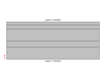
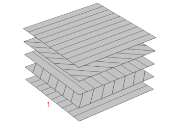
You can do that by creating Layer Cross Section Preview () and Layer Stack Preview () plots. An example of a layer cross section plot showing a 2D cross section of a laminate having is shown in Figure 3-6. The thickness of each layer is visible. An example of a layer stack preview plot showing the stacking sequence is shown in Figure 3-7.
Figure 3-6: Example of a layer cross section preview plot showing a composite laminate having 5 layers with different thickness values.
Figure 3-7: Example of a layer stack preview plot showing a composite laminate having 5 layers with stacking sequence [0/45/90/-45/0].
Note that in the layer stack preview plot, the distance between any two layers are always the same and it does not reflect the actual thickness of the layers.
Since the preview plots are used for variety of composite laminates having different combination of number of layers, thickness values, and stacking sequence, it is possible to customize the plot settings in terms of changing the thickness to width ratio or the distance between the orientation lines. It is also possible to switch off the orientation lines and labels.
In the COMSOL Multiphysics Reference Manual: