Contact Analysis Theory

In the augmented Lagrangian method, the system of equations is solved in a segregated way. Augmentation components are introduced for the contact pressure Tn and the components Tti of the friction traction vector Tt. An additional iteration level is added where the usual displacement variables are solved separated from the contact pressure and traction variables. The algorithm repeats this procedure until it fulfills a convergence criterion.

In the penalty method, no extra degrees of freedom are needed for the contact pressure or the friction traction vector. These results are just computed from the displacements and the penalty stiffness. This means that no special solver strategies are necessary.

In the following equations F is the deformation gradient matrix. When looking at expressions evaluated on the destination boundaries, the expression map (E) denotes the value of the expression E evaluated at a corresponding source point, and g is the current gap distance between the destination and source boundary.

Both the contact map operator map (E) and the gap distance variable are defined by the contact element elcontact. For each destination point where the operator or gap is evaluated, a corresponding source point is sought by searching in the direction normal to the destination boundary.

Before the boundaries come in contact, the source point found is not necessarily the point on the source boundary closest to the destination point. However, as the boundaries approach one another, the source point converges to the closest point as the gap distance approaches zero.

It is possible to add an offset value both to the source (osrc), and to the destination (odst). If an offset is used, the gap will be computed with the geometry treated as larger (or smaller, in the case of a negative offset) than what is actually modeled. The offset is given in a direction normal to the boundary. It can vary along the geometry, and may also vary in time (or by parameter value when using the continuation solver).

The effective gap distance dg used in the analysis is thus

The correction of the source side offset is necessary since the normal on the source side is not necessarily pointing towards the current point on the destination. When in contact, the normals will be exactly opposite.

In some cases, the discretization caused by the meshing of curved boundaries will give small irregularities in the gap values. You can then choose to adjust the gap by the computed gap value in the initial configuration, ginit. In this case, the effective gap distance is

When including friction in the contact problem, it is important to keep track of not only the gap in the normal direction, but also the slip between the boundaries in the tangential direction. The slip s since the last converged step is defined as

where the index ‘m’ indicates that the coordinates are taken as the mapped coordinates from the source side,

and Xm,old is the value of Xm in the last converged time or parameter step. The coordinates are material (undeformed) coordinates. The slip vector is thus approximated using a backward Euler step. The deformation gradient F contains information about the local rotation and stretching.

Using the special gap distance variable (solid.gap), the penalized contact pressure Tnp is defined on the destination boundary as

pn is the user-defined normal penalty factor.

The penalized friction traction Ttp is defined on the destination boundary as:

where Tt,trial is defined as

In Equation 3-57, pt is the user-defined friction traction penalty factor. The critical sliding resistance, Tt,crit, is defined as

In Equation 3-58, μ is the friction coefficient, Tcohe is the user-defined cohesion sliding resistance, and Tt,max is the user-defined maximum friction traction.

In the following equation δ is the variation (represented by the test() operator in COMSOL Multiphysics). The contact interaction gives the following contribution to the virtual work on the destination boundary:

where wcn and wct are contact help variables defined as:

where i is the augmented solver iteration number and γfric is a Boolean variable stating if the parts are in contact or not.

The penalty algorithm is essentially based on the insertion of a stiff spring between the contacting boundaries. The penalty factor can be interpreted as the stiffness of that spring. A high value of the stiffness fulfills the contact conditions more accurately, but if it is too high, it makes the problem ill-conditioned and unstable. The contact pressure in the normal direction is computed as

where dg is the effective gap distance, pn is the penalty factor, and p0 is the pressure at zero gap. The latter parameter can be used to reduce the overclosure between the contacting boundaries if an estimate to the contact pressure is known. In the default case, when p0 = 0, there must always be some overclosure (a negative gap) in order for a contact pressure to develop.

In case of friction, the tangential force Tt is computed as

This can be viewed as a tangential spring giving a force proportional to the sliding distance. The penalty factor pt can be identified as the spring constant. The sticking condition is thus replaced by a stiff spring, so that there is a small relative movement even if the force required for sliding is not exceeded.

The definition of Tt,crit depends on the algorithm used for computing the normal contact.

The same notation as for the description of the augmented Lagrangian method above is used.

The springs between the contacting boundaries are added using weak expressions on the destination boundary.

The friction model is either no friction or Coulomb friction.

The frictional coefficient μ is defined as

where μs is the static frictional coefficient, μd is the dynamic frictional coefficient, vs is the slip velocity, and αdcf is a decay coefficient.

Since the contact model always makes use of the geometric nonlinearity assumption, the contact pressure and the friction force represent, respectively, the normal and tangential components of the nominal traction. This is the force density with components in the current configuration (that is, on the spatial frame) but related to the undeformed area of the corresponding surface element.

You can model a situation where two boundaries stick together once the get into contact by adding an Adhesion subnode to . Adhesion can be modeled when the penalty contact method is used. The adhesion formulation can be viewed as if a thin elastic layer is placed between the source and destination boundaries when adhesion is activated.

The adhesion starts acting when the adhesion criterion is met in the previous time or parameter step. An auxiliary degree of freedom located at Gauss points is used as an indicator to whether the adhesion criterion has been met or not.

When adhesion is active, the tensile stress σn in the normal direction is computed from the effective gap dg as

The default value for the stiffness in the normal direction Kp is the penalty stiffness of the contact condition, but you can also enter it explicitly. In compression, the penalty stiffness is always used. This leads to a bilinear stiffness in the normal direction when is .

The shearing deformation is resisted using a shear stiffness

, related to the normal stiffness by

where

is a coefficient with the default value 0.17. This coefficient can either be input explicitly, or be computed from a Poisson’s ratio. A plane strain assumption is used for this conversion, giving

The shear traction is proportional to the relative deformation between the source and destination boundaries measured from the position when the adhesion criterion was first fulfilled, so that

where s is the slip vector.

When adhesion is active, it is possible to break the bond between the source and destination boundaries by specifying a . Three different such decohesion laws are available.

The decohesion behavior in both tension or shear is based on two quantities, the maximum stress and the energy release rate. Tearing in the normal direction is called mode I, and shear is called mode II. In the theory below a subscript i can take the values I and II.

Up to the maximum stress, the adhesive layer is linearly elastic. At higher deformation, the stress decreases, and a damage is assumed to have occurred. The damage function is a scalar function of the maximum relative displacement between the two boundaries. The stiffness in the damaged state is permanently reduced, even on unloading.

In general, the stress state is a combination of tension and shear, so the data for the two modes must be combined into a multiaxial decohesion rule. For two of the decohesion laws you can specify details of the multiaxial behavior.

As a measure of the displacement in the adhesive layer, the mixed mode relative displacement um, is defined as weighted combination of the normal direction displacement uI and the tangential displacement uII.

In this expression, the notation

has been used. This is the displacement which is compared with the various mixed mode failure displacements described below.

In the linear separation law, the decreasing part of the stress vs. displacement curve is linear. The graph in Figure 3-18 is generic, and valid both for mode I and mode II.

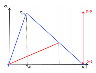
The failure initiation displacement ui0 for each mode is determined from the maximum stress and the elastic stiffness, as

The decohesion displacement uif for each mode is implicitly determined from the given energy release rate (which is the area under the stress vs. displacement curve):

The mixed mode failure initiation displacement is then defined as

The implication is that compressive displacements are ignored, and only tensile and tangential displacements contribute.

The final mixed mode failure displacement depends on the selected . The failure criterion is defined as

whereas the failure criterion is defined as

The exponent η is called the .

From these relations, the total decohesion failure displacement in the mixed mode can be computed. For a power law criterion, the expression is

For the Benzeggagh-Kenane criterion, the corresponding expression is

The damage function can be described as

The secant stiffness of the damaged adhesive layer (indicated by the red line in Figure 3-18) is

The polynomial separation law differs from the linear separation law in that the decreasing part of the stress curve is represented by a cubic polynomial. This polynomial is chosen so that it has zero slope in both ends, which means that the secant stiffness does not have any discontinuities. The area under the cubic function is the same as that of the linear function when the failure displacement uif is the same. That is, for a given energy release rate Gic, the same uif is obtained.

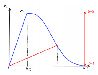
All expressions presented under Linear separation law are still valid except the damage function, which now is

The multilinear separation law introduces a region of constant stress, similar to a perfectly plastic material model, as shown in Figure 3-20.

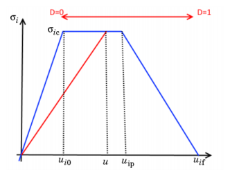
This law requires one more material parameter λ, describing the width of the “plastic” region. The λ is the ratio between the plastic (constant stress) part of Gic and the total “inelastic” part of Gic: