Rigid Domain Material Model

A Rigid Domain, or a rigid body, is an idealization of a body in which the deformation is neglected. In other words, the distance between any two given points of a rigid body remains constant in time regardless of any external forces acting on it. An object can be assumed to be perfectly rigid if its flexibility can be neglected in comparison with other flexibilities in the system, and when there is no need to compute the stress in the object.


	Rigid Domain is available as a material model both in the Solid Mechanics, Shell, Beam, and Multibody Dynamics interfaces. This theory section applies to all interfaces. There are some minor differences between the versions of the Rigid Domain which will be described as they appear. A Rigid Domain can consist of a selection of several geometrical domains. These domains will act as a single rigid object, irrespective of whether they are geometrically connected or not. Adjacent geometrical objects selected in different Rigid Domains nodes are independent, and can even penetrate each other.

The rigid domain is a material model, which is mutually exclusive to all other material models. The only material property needed is the mass density.

Rigid Domain Kinematics

When a body is rigid, it is sufficient to describe the motion of at least three non-collinear particles. It is then possible to reconstruct the motion of all other particles in the body. Usually a mathematically more convenient, but equivalent, approach is used. The motion of the whole body is represented by:

•

The linear motion of the body. The motion of one of the particles of the body, chosen as a reference point (often coinciding with the center of mass).

•

The angular motion (also known as orientation or attitude) of the body.

The degrees of freedom needed to represent the linear and angular motion are known as rigid body translation and rigid body rotation degrees of freedom.

In 2D, this is represented by two in-plane translations and the rotation around the z-axis.

In 3D the situation is more complex. Six degrees of freedom are necessary. They are usually selected as three translations and three parameters for the rotation. For finite rotations any choice of three rotation parameters is however singular at some specific set of angles. For this reason, a four-parameter quaternion representation is used for the rotations in COMSOL Multiphysics. Thus, each rigid domain in 3D actually has seven degrees of freedom: three for the translation, and four for the rotation. The quaternion parameters are called a, b, c, and d, respectively. These four parameters are not independent, so an extra equation stating that

is added.

The connection between the quaternion parameters and the rotation matrix R is:

For the geometrically linear case, the quaternion constraint and the rotation matrix definition are reduced to:

In 2D, the rotational degree of freedom is the angle of rotation about the z-axis

, and its relation with the rotation matrix R is:

For the geometrically linear case, the 2D rotation matrix is reduced to:

Under translation and rotation of a rigid domain, the complete expression for the displacement of any point on the rigid body is given by:

where X are the material coordinates of any point in the rigid domain,

is the center of mass of the rigid domain, u is the translation vector at the center of mass, and I is the identity matrix.

The rigid body displacement at the center of mass (u) are degrees of freedom. Thus the rigid body translational velocity and acceleration can be evaluated by directly taking the time derivatives of u. In the time domain it can be expressed as:

In the frequency domain, they can be expressed in terms of frequency (ω):

The same is true for the rotation in 2D since the rigid body rotation

is the degree of freedom. The rigid body angular velocity and acceleration can be evaluated by directly taking the time derivatives of

In 3D, the situation is different and the total rotation of the rigid domain can be presented as a function of quaternion:

The parameter a can be considered as measuring the rotation, while b, c, and d can be interpreted as the orientation of the rotation vector. For small rotations, this relation simplifies to:

The angular velocity of the rigid domain is computed as:

Here

is the conjugate of q, and the symbol

denotes quaternion multiplication.

The angular acceleration of the rigid domain can be evaluated by taking the time derivative of the angular velocity.

Rigid Domain Dynamics

The governing equation for a rigid domain can be written as a balance between the inertial (internal) forces and applied external forces. A rigid domain has only one internal force, the inertial force. This means that only the mass density of a domain is required to define the rigid domain material model.

The inertial forces and inertial moments about the center of mass are:

where

and

are the linear and angular accelerations of a rigid domain.

The inertial properties mass (m) and moment of inertia tensor (I) of a rigid domain are computed as:

where

and

are the identity matrix and the center of mass of a rigid domain, respectively. The special case for the Shell interface is described in Rigid Domain for Shells.

In 2D, the expressions for inertial forces, inertial moments, and moment of inertia reduce to:

where the volume integration has been replaced by an area integration multiplied by the out-of-plane thickness h.

The equations of motion for the rigid domain are:

and

Here, the subscripts ‘I’ and ‘ext’ denotes inertial and external forces respectively, and R is the current rotation matrix. The inertial forces are contributions from Mass and Moment of Inertia nodes.

In 2D, the moment equations are simplified to the scalar equation

Initial Value

As a Rigid Domain is a separate material model, it overrides the default Linear Elastic Material model and its default Initial Values node. The initial values are given in a separate Initial Values subnode for each Rigid Domain.


	In the Multibody Dynamics interface version of the Rigid Domain, it is also possible to get initial values for all domains from the interface level Initial Values section. This is the default option. The Initial Values subnode is only present under Rigid domain if Locally defined has been selected. If many rigid domains are present in a system and the have the same initial values, then it is often better to define initial values at the interface level once and to reference it in all features.

The initial values for the rigid body translation, rigid body rotation, and the first time derivatives can be prescribed about any point—a center of rotation—in a selected coordinate system. The center of rotation can be defined using

•

The center of mass of the rigid domain

•

Global coordinates of the center of rotation

•

The centroid of a set of selected entities (boundaries, edges, or points)

Given the initial values of translation (u), rotation (

), translational velocity (

) and angular velocity (

) about a center of rotation (

), the rigid body displacement and quaternion degrees of freedom are initialized as:

In 2D, the expressions for the initial values reduce to:

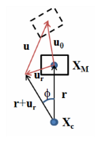
The variable ur is the translation at the center of mass due to a rotation around the center of rotation, and is thus zero when the two points coincide. In the case that you are entering the data using a separate center of rotation, you must pay special attention to how the initial displacement and velocity are composed if initial rotations and rotational velocities are present.

Figure 3-16: Initial displacement of a rigid body

Mass and Moment of Inertia

Sometimes a rigid domain needs the added effect of an associated abstract rigid object, which is physically not modeled and where the inertial properties are known. You can model this using Mass and Moment of Inertia, where the inertial properties of this abstract domain (center of mass, mass, and moment of inertia tensor) can be directly entered.

The formulation for an abstract rigid object is similar to the physical rigid domain with these exceptions:

•

The inertial properties of the abstract rigid object are input by the user instead of being computed from a physical domain.

•

No extra degrees of freedom are created. The inertial forces generated by this feature will be computed based on the distance from the center of gravity of the rigid domain to which it belongs, and the values of the degrees of freedom there.

The inertial force contributions are

where Xmc is the vector from the center of mass of the rigid domain (XM) to the center of mass of this contribution (Xm),

The inertial moment contributions are

In 2D, there is only a scalar moment contribution:

Constraints

The constraints for a rigid domain are different in nature than those applied to flexible domain. In a flexible domain, a constraint can be applied at various entity levels: domains, boundaries, edges, or points. Since the degrees of freedom of the rigid domain are global and present only at the center of mass, boundary conditions are used to constrain these global degrees of freedom, which is why a global selection is needed.


	The constraints used for a flexible domain, for example Fixed Constraint, Prescribed Displacement, Rigid Connector, or Attachment, are not applicable to a rigid domain. In a rigid domain the Prescribed Displacement/Rotation or Fixed Constraint subnode is used instead to constrain its degrees of freedom.

The node can be used to:

•

Prescribe the displacement components in arbitrary directions at a given point.

•

Constrain rotations in arbitrary directions.

•

Prescribe a non-zero rotation around an arbitrary axis.

The displacement and rotation can be prescribed in a selected coordinate system about an arbitrary center of rotation. The center of rotation can be defined using

•

The center of mass of the rigid domain.

•

Global coordinates of the center of rotation.

•

The centroid of a set of selected entities (boundaries, edges, or points).

The displacement at the center of rotation is computed as:

(3-50)

The components of this displacement vector are prescribed individually in the selected coordinate system. Through Equation 3-50, a constraint on a translation will impose a relation between translational and rotational degrees of freedom if the center of rotation differs from the center of mass.

To prescribe the rotation in 3D, the imaginary part of the quaternion is prescribed as:

where

and

are the axis of rotation and angle of rotation respectively.

In 2D, the out-of-plane rotation angle is directly constrained to the prescribed value of the rotation.

Loads

The loads available for a flexible domain can also be used for a rigid domain. In addition to these boundary conditions, a rigid domain also has global subnodes for applying forces and moments. If you use , a force and its location can be prescribed in a selected coordinate system. A force implicitly also contributes to the moment unless it is applied at the center of mass of a rigid domain. If an node is used, a moment can be prescribed in a selected coordinate system.

Connecting to Other Bodies

When a rigid domain and a flexible domain share a boundary (Shell: edge, Beam: point), the connection is automatic. All displacements on the flexible domain are controlled by the degrees of freedom of the rigid domain, so that

where X is a coordinate on the boundary. If rotational degrees of freedom are present, which is the case in the Shell and Beam interfaces, the rotations are set equal to those of the rigid domain.


	In the Multibody Dynamics interface, a rigid domain can be also be connected to another rigid or flexible domain using joints. A rigid component can be directly selected in the joints to establish a connection. This stands in contrast to a flexible component, which needs an attachment. A Rigid Domain which contains a selection of several geometrical domains will act as a single rigid object. Adjacent domains selected in different Rigid Domains nodes are independent objects.